6. Process or Product Monitoring and Control
6.6. Case Studies in Process Monitoring
6.6.1. Lithography Process

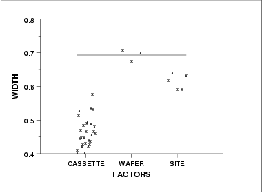
6.6.1.2.

Graphical Representation of the Data

The first step in analyzing the data is to generate some simple plots of the response and then of the response versus the various factors.

4-Plot of Data

Interpretation

This 4-plot shows the following.

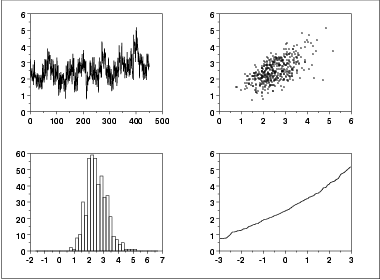
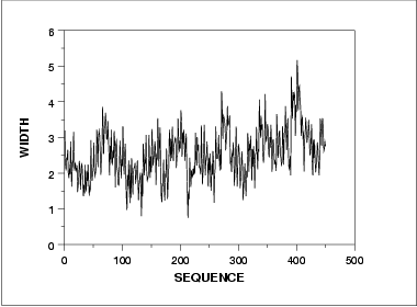
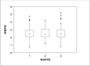
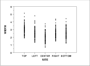
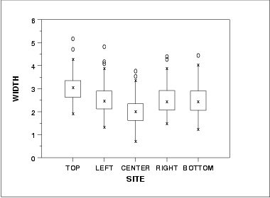
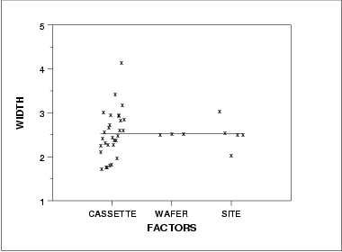
1. The run sequence plot (upper left) indicates that the location and scale are not constant over time. This indicates that the three factors do in fact have an effect of some kind.
2. The lag plot (upper right) indicates that there is some mild autocorrelation in the data. This is not unexpected as the data are grouped in a logical order of the three factors (i.e., not randomly) and the run sequence plot indicates that there are factor effects.
3. The histogram (lower left) shows that most of the data fall between 1 and 5, with the center of the data at about 2.2.
4. Due to the non-constant location and scale and autocorrelation in the data, distributional inferences from the normal probability plot (lower right) are not meaningful.

The run sequence plot is shown at full size to show greater detail. In addition, a numerical summary of the data is generated.

Run Sequence Plot of Data

Numerical Summary

Sample size = 450 Mean = 2.53228 Median = 2.45334 Minimum = 0.74655 Maximum = 5.16867 Range = 4.42212 Stan. Dev. = 0.69376 Autocorrelation = 0.60726 We are primarily interested in the mean and standard deviation. From the summary, we see that the mean is 2.53 and the standard deviation is 0.69.

Plot response against individual factors	The next step is to plot the response against each individual factor. For comparison, we generate both a scatter plot and a box plot of the data. The scatter plot shows more detail. However, comparisons are usually easier to see with the box plot, particularly as the number of data points and groups become larger.
Scatter plot of width versus cassette
Box plot of width versus cassette
Interpretation	We can make the following conclusions based on the above scatter and box plots. There is considerable variation in the location for the various cassettes. The medians vary from about 1.7 to 4. There is also some variation in the scale. There are a number of outliers.
Scatter plot of width versus wafer
Box plot of width versus wafer
Interpretation	We can make the following conclusions based on the above scatter and box plots. The locations for the three wafers are relatively constant. The scales for the three wafers are relatively constant. There are a few outliers on the high side. It is reasonable to treat the wafer factor as homogeneous.
Scatter plot of width versus site
Box plot of width versus site
Interpretation	We can make the following conclusions based on the above scatter and box plots. There is some variation in location based on site. The center site in particular has a lower median. The scales are relatively constant across sites. There are a few outliers.
DOE mean and sd plots	We can use the DOE mean plot and the DOE standard deviation plot to show the factor means and standard deviations together for better comparison.
DOE mean plot
DOE sd plot
Summary	The above graphs show that there are differences between the lots and the sites. There are various ways we can create subgroups of this dataset: each lot could be a subgroup, each wafer could be a subgroup, or each site measured could be a subgroup (with only one data value in each subgroup). Recall that for a classical Shewhart means chart, the average within subgroup standard deviation is used to calculate the control limits for the means chart. However, with a means chart you are monitoring the subgroup mean-to-mean variation. There is no problem if you are in a continuous processing situation - this becomes an issue if you are operating in a batch processing environment. We will look at various control charts based on different subgroupings in 6.6.1.3.