6. Process or Product Monitoring and Control
6.6. Case Studies in Process Monitoring
6.6.1. Lithography Process

6.6.1.3.

Subgroup Analysis

Control charts for subgroups

The resulting classical Shewhart control charts for each possible subgroup are shown below.

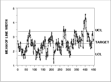
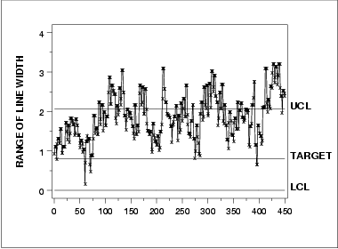
Site as subgroup

The first pair of control charts use the site as the subgroup. However, since site has a subgroup size of one we use the control charts for individual measurements. A moving average and a moving range chart are shown.

Moving average control chart

Moving range control chart

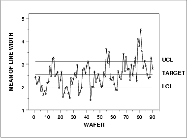
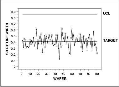
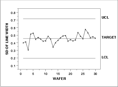
Wafer as subgroup

The next pair of control charts use the wafer as the subgroup. In this case, the subgroup size is five. A mean and a standard deviation control chart are shown.

Mean control chart

SD control chart

There is no LCL for the standard deviation chart because of the small subgroup size.

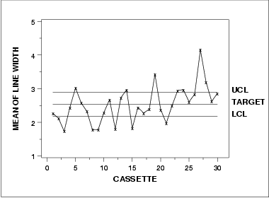
Cassette as subgroup

The next pair of control charts use the cassette as the subgroup. In this case, the subgroup size is 15. A mean and a standard deviation control chart are shown.

Mean control chart

SD control chart

Interpretation

Which of these subgroupings of the data is correct? As you can see, each sugrouping produces a different chart. Part of the answer lies in the manufacturing requirements for this process. Another aspect that can be statistically determined is the magnitude of each of the sources of variation. In order to understand our data structure and how much variation each of our sources contribute, we need to perform a variance component analysis. The variance component analysis for this data set is shown below.

Component	Variance Component Estimate
Cassette	0.2645
Wafer	0.0500
Site	0.1755

Variance Component Estimation

If your software does not generate the variance components directly, they can be computed from a standard analysis of variance output by equating mean squares (MS) to expected mean squares (EMS).

The sum of squares and mean squares for a nested, random effects model are shown below.

                      Degrees of    Sum of
Source                 Freedom      Squares   Mean Squares
--------------------  ----------  ---------   ------------
Cassette                  29      127.40293      4.3932 
Wafer(Cassette)           60       25.52089      0.4253
Site(Cassette, Wafer)    360       63.17865      0.1755

The expected mean squares for cassette, wafer within cassette, and site within cassette and wafer, along with their associated mean squares, are the following.

4.3932 = (3*5)*Var(cassettes) + 5*Var(wafer) + Var(site)
0.4253 = 5*Var(wafer) + Var(site)
0.1755 = Var(site)

Solving these equations, we obtain the variance component estimates 0.2645, 0.04997, and 0.1755 for cassettes, wafers, and sites, respectively.

All of the analyses in this section can be completed using R code. The reader can download the data as a text file.