6. Process or Product Monitoring and Control
6.6. Case Studies in Process Monitoring
6.6.2. Aerosol Particle Size

6.6.2.4.

Model Validation

Residuals

After fitting the model, we should check whether the model is appropriate.

As with standard non-linear least squares fitting, the primary tool for model diagnostic checking is residual analysis.

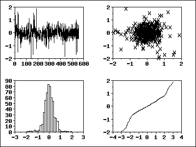
4-Plot of Residuals from ARIMA(2,1,0) Model

The 4-plot is a convenient graphical technique for model validation in that it tests the assumptions for the residuals on a single graph.

Interpretation of the 4-Plot

We can make the following conclusions based on the above 4-plot.

1. The run sequence plot shows that the residuals do not violate the assumption of constant location and scale. It also shows that most of the residuals are in the range (-1, 1).
2. The lag plot indicates that the residuals are not autocorrelated at lag 1.
3. The histogram and normal probability plot indicate that the normal distribution provides an adequate fit for this model.

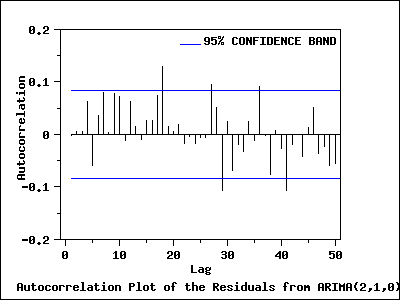
Autocorrelation Plot of Residuals from ARIMA(2,1,0) Model

In addition, the autocorrelation plot of the residuals from the ARIMA(2,1,0) model was generated.

Interpretation of the Autocorrelation Plot

The autocorrelation plot shows that for the first 25 lags, all sample autocorrelations expect those at lags 7 and 18 fall inside the 95% confidence bounds indicating the residuals appear to be random.

Ljung-Box Test for Randomness for the ARIMA(2,1,0) Model

Instead of checking the autocorrelation of the residuals, portmanteau tests such as the test proposed by Ljung and Box (1978) can be used. In this example, the test of Ljung and Box indicates that the residuals are random at the 95% confidence level and thus the model is appropriate. Dataplot generated the following output for the Ljung-Box test.

               LJUNG-BOX TEST FOR RANDOMNESS
  
 1. STATISTICS:
       NUMBER OF OBSERVATIONS      =      559
       LAG TESTED                  =       24
       LAG 1 AUTOCORRELATION       =  -0.1012441E-02
       LAG 2 AUTOCORRELATION       =   0.6160716E-02
       LAG 3 AUTOCORRELATION       =   0.5182213E-02
  
    LJUNG-BOX TEST STATISTIC       =    31.91066
  
 2. PERCENT POINTS OF THE REFERENCE CHI-SQUARE DISTRIBUTION
    (REJECT HYPOTHESIS OF RANDOMNESS IF TEST STATISTIC VALUE
    IS GREATER THAN PERCENT POINT VALUE)
    FOR LJUNG-BOX TEST STATISTIC
       0          % POINT    =          0.
       50         % POINT    =    23.33673
       75         % POINT    =    28.24115
       90         % POINT    =    33.19624
       95         % POINT    =    36.41503
       99         % POINT    =    42.97982
  
  
 3. CONCLUSION (AT THE 5% LEVEL):
    THE DATA ARE RANDOM.

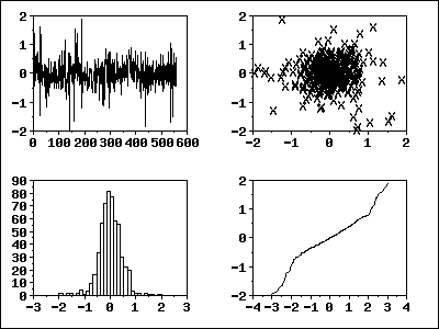
4-Plot of Residuals from ARIMA(0,1,1) Model

The 4-plot is a convenient graphical technique for model validation in that it tests the assumptions for the residuals on a single graph.

Interpretation of the 4-Plot from the ARIMA(0,1,1) Model

We can make the following conclusions based on the above 4-plot.

1. The run sequence plot shows that the residuals do not violate the assumption of constant location and scale. It also shows that most of the residuals are in the range (-1, 1).
2. The lag plot indicates that the residuals are not autocorrelated at lag 1.
3. The histogram and normal probability plot indicate that the normal distribution provides an adequate fit for this model.

This 4-plot of the residuals indicates that the fitted model is an adequate model for these data.

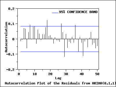
Autocorrelation Plot of Residuals from ARIMA(0,1,1) Model

The autocorrelation plot of the residuals from ARIMA(0,1,1) was generated.

Interpretation of the Autocorrelation Plot

Similar to the result for the ARIMA(2,1,0) model, it shows that for the first 25 lags, all sample autocorrelations expect those at lags 7 and 18 fall inside the 95% confidence bounds indicating the residuals appear to be random.

Ljung-Box Test for Randomness of the Residuals for the ARIMA(0,1,1) Model

The Ljung and Box test is also applied to the residuals from the ARIMA(0,1,1) model. The test indicates that the residuals are random at the 99% confidence level, but not at the 95% level.

Dataplot generated the following output for the Ljung-Box test.

               LJUNG-BOX TEST FOR RANDOMNESS
  
 1. STATISTICS:
       NUMBER OF OBSERVATIONS      =      559
       LAG TESTED                  =       24
       LAG 1 AUTOCORRELATION       =  -0.1280136E-01
       LAG 2 AUTOCORRELATION       =  -0.3764571E-02
       LAG 3 AUTOCORRELATION       =   0.7015200E-01
  
    LJUNG-BOX TEST STATISTIC       =    38.76418
  
 2. PERCENT POINTS OF THE REFERENCE CHI-SQUARE DISTRIBUTION
    (REJECT HYPOTHESIS OF RANDOMNESS IF TEST STATISTIC VALUE
    IS GREATER THAN PERCENT POINT VALUE)
    FOR LJUNG-BOX TEST STATISTIC
       0          % POINT    =          0.
       50         % POINT    =    23.33673
       75         % POINT    =    28.24115
       90         % POINT    =    33.19624
       95         % POINT    =    36.41503
       99         % POINT    =    42.97982
  
  
 3. CONCLUSION (AT THE 5% LEVEL):
    THE DATA ARE NOT RANDOM.

Summary

Overall, the ARIMA(0,1,1) is an adequate model. However, the ARIMA(2,1,0) is a little better than the ARIMA(0,1,1).