LPOPPF

LPOPPF (LET)

Library Function

Compute the Lagrange-Poisson percent point function.

The Lagrange Poisson distribution has probability mass function

with and denoting the shape parameters.

The cumulative distribution function is computed by summing the probability mass function. The percent point function is the inverse of the cumulative distribution function and is obtained by computing the cumulative distribution function until the specified probability is reached.

LET <y> = LPOPPF(<p>,<lambda>,<theta>)>
                        <SUBSET/EXCEPT/FOR qualification>
where <p> is a variable, number, or parameter in the interval (0,1);
            <lambda> is a number or parameter in the range (0,1) that specifies the first shape parameter;
            <theta> is a positive number or parameter that specifies the second shape parameter;
            <y> is a variable or a parameter where the computed Lagrange-Poisson ppf value is stored;
and where the <SUBSET/EXCEPT/FOR qualification> is optional.

LET A = LPOPPF(0.95,0.5,3)
LET Y = LPOPPF(P,0.3,2)
PLOT LPOPPF(P,0.3,2) FOR P = 0 0.01 0.99

None

None

LPOCDF	= Compute the Lagrange-Poisson cumulative distribution function.
LPOPDF	= Compute the Lagrange-Poisson probability mass function.
BTAPDF	= Compute the Borel-Tanner probability mass function.
LOSPDF	= Compute the lost games probability mass function.
POIPDF	= Compute the Poisson probability mass function.
HERPDF	= Compute the Hermite probability mass function.
BINPDF	= Compute the binomial probability mass function.
NBPDF	= Compute the negative binomial probability mass function.
GEOPDF	= Compute the geometric probability mass function.

Johnson, Kotz, and Kemp (1992), "Univariate Discrete Distributions", Second Edition, Wiley, pp. 394-400.

P. C. Consul (1989), "Generalized Poisson Distributions", Dekker, New York.

Distributional Modeling

2006/6

 
title size 3
tic label size 3
label size 3
legend size 3
height 3
multiplot scale factor 1.5
x1label displacement 12
y1label displacement 17
.
multiplot corner coordinates 0 0 100 95
multiplot scale factor 2
label case asis
title case asis
case asis
tic offset units screen
tic offset 3 3
title displacement 2
x1label Probability
y1label X
.
xlimits 0 1
major xtic mark number 6
minor xtic mark number 3
.
multiplot 2 2
.
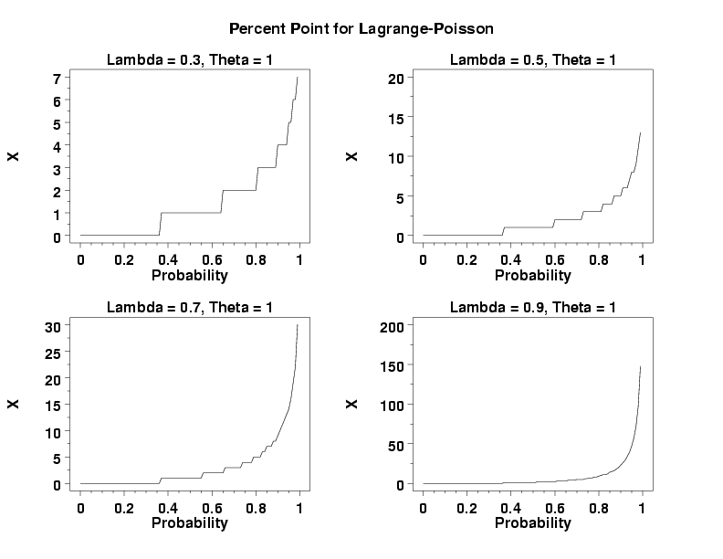
title Lambda = 0.3, Theta = 1
plot lpoppf(p,0.3,1) for p = 0  0.01  0.99
.
title Lambda = 0.5, Theta = 1
plot lpoppf(p,0.5,1) for p = 0  0.01  0.99
.
title Lambda = 0.7, Theta = 1
plot lpoppf(p,0.7,1) for p = 0  0.01  0.99
.
title Lambda = 0.9, Theta = 1
plot lpoppf(p,0.9,1) for p = 0  0.01  0.99
.
end of multiplot
.
justification center
move 50 97
text Percent Point for Lagrange-Poisson