
|
GLSPDFName:

with Note that there are several distributions in the literature that are called the generalized logarithmic series distribution. We are using the definition given in Consul and Famoye (see References below).
<SUBSET/EXCEPT/FOR qualification> where <x> is a positive integer variable, number, or parameter; <theta> is a number, parameter, or variable in the range (0,1) that specifies the first shape parameter; <beta> is a number, parameter, or variable that specifies the second shape parameter; <y> is a variable or a parameter (depending on what <x> is) where the computed generalized logarithmic series pdf value is stored; and where the <SUBSET/EXCEPT/FOR qualification> is optional.
LET Y = GLSPDF(X,0.3,1.6) PLOT GLSPDF(X,0.3,1.6) FOR X = 1 1 20
LET THETA = <value> LET BETA = <value> LET Y = GENERALIZED LOGARITHMIC SERIES ... RANDOM NUMBERS FOR I = 1 1 N
GENERALIZED LOGARITHMIC SERIES PROBABILITY PLOT Y
GENERALIZED LOGARITHMIC SERIES CHI-SQUARE ... To obtain the method of moment estimates, the mean and ones frequency estimates, and the maximum likelihood estimates of theta and beta, enter the command
GENERALIZED LOGARITHMIC SERIES MAXIMUM LIKELIHOOD Y2 X2
The method of moment estimate of

with
The moment estimate of

The proportion of ones and sample mean method estimate of

with
The proportion of ones and sample mean estimate of

The maximum likelihood estimates of

with k, n, and nx denoting the number of classes, the total sample size, and the count for the xth class, respectively.
You can generate estimates of
LET THETA2 = <value> LET BETA1 = <value> LET BETA2 = <value> GENERALIZED LOGARITHMIC SERIES KS PLOT Y GENERALIZED LOGARITHMIC SERIES KS PLOT Y2 X2 GENERALIZED LOGARITHMIC SERIES KS PLOT ... Y3 XLOW XHIGH GENERALIZED LOGARITHMIC SERIES PPCC PLOT Y GENERALIZED LOGARITHMIC SERIES PPCC PLOT Y2 X2 GENERALIZED LOGARITHMIC SERIES PPCC PLOT ... Y3 XLOW XHIGH
The default values of theta1 and theta2 are 0.05 and 0.95,
respectively. The default values for beta1 and beta2 are
1.05 and 5, respectively. Note that values of
Due to the discrete nature of the percent point function for discrete distributions, the ppcc plot will not be smooth. For that reason, if there is sufficient sample size the KS PLOT (i.e., the minimum chi-square value) is typically preferred. However, it may sometimes be useful to perform one iteration of the PPCC PLOT to obtain a rough idea of an appropriate neighborhood for the shape parameters since the minimum chi-square statistic can generate extremely large values for non-optimal values of the shape parameters. Also, since the data is integer values, one of the binned forms is preferred for these commands.
Famoye (1995), "On Certain Methods of Estimation for Generalized Logarithmic Series Distribution", Journal of Applied Statistical Sciences, 2, pp. 103-117.
title size 3
tic label size 3
label size 3
legend size 3
height 3
x1label displacement 12
y1label displacement 15
.
multiplot corner coordinates 0 0 100 95
multiplot scale factor 2
label case asis
title case asis
case asis
tic offset units screen
tic offset 3 3
title displacement 2
y1label Probability Mass
x1label X
.
ylimits 0 1
major ytic mark number 6
minor ytic mark number 3
xlimits 0 20
line blank
spike on
.
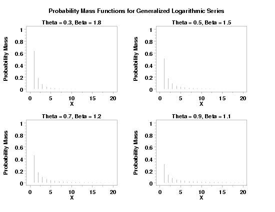
multiplot 2 2
.
title Theta = 0.3, Beta = 1.8
plot glspdf(x,0.3,1.8) for x = 1 1 20
.
title Theta = 0.5, Beta = 1.5
plot glspdf(x,0.5,1.5) for x = 1 1 20
.
title Theta = 0.7, Beta = 1.2
plot glspdf(x,0.7,1.2) for x = 1 1 20
.
title Theta = 0.9, Beta = 1.1
plot glspdf(x,0.9,1.1) for x = 1 1 20
.
end of multiplot
.
justification center
move 50 97
text Probability Mass Functions for Generalized Logarithmic Series

Program 2:
LET THETA = 0.7
LET BETA  = 1.2
LET Y = GENERALIZED LOGARITHMIC SERIES RANDOM NUMBERS ...
        FOR I = 1 1 500
.
LET Y3 XLOW XHIGH = INTEGER FREQUENCY TABLE Y
CLASS LOWER 0.5
CLASS WIDTH 1
LET AMAX = MAXIMUM Y
LET AMAX2 = AMAX + 0.5
CLASS UPPER AMAX2
LET Y2 X2 = BINNED Y
.
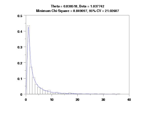
GENERALIZED LOGARITHMIC SERIES MLE Y
RELATIVE HISTOGRAM Y2 X2
LIMITS FREEZE
PRE-ERASE OFF
LINE COLOR BLUE
PLOT GLSPDF(X,THETAML,BETAML) FOR X = 0  1  AMAX
LIMITS
PRE-ERASE ON
LINE COLOR BLACK
LET THETA = THETAML
LET BETA  = BETAML
GENERALIZED LOGARITHMIC SERIES CHI-SQUARE GOODNESS OF FIT ...
    Y3 XLOW XHIGH
CASE ASIS
JUSTIFICATION CENTER
MOVE 50 97
TEXT Theta = ^THETAML, Beta = ^BETAML
MOVE 50 93
TEXT Minimum Chi-Square = ^STATVAL, 95% CV = ^CUTUPP95
.
LABEL CASE ASIS
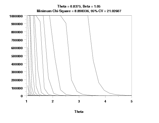
X1LABEL Theta
Y1LABLE Minimum Chi-Square
GENERALIZED LOGARITHMIC SERIES KS PLOT Y3 XLOW XHIGH
LET THETA = SHAPE1
LET BETA  = SHAPE2
GENERALIZED LOGARITHMIC SERIES CHI-SQUARE GOODNESS OF FIT ...
    Y3 XLOW XHIGH
JUSTIFICATION CENTER
MOVE 50 97
TEXT Theta = ^THETA, Beta = ^BETA
MOVE 50 93
TEXT Minimum Chi-Square = ^MINKS, 95% CV = ^CUTUPP95

                   CHI-SQUARED GOODNESS-OF-FIT TEST

 NULL HYPOTHESIS H0:      DISTRIBUTION FITS THE DATA
 ALTERNATE HYPOTHESIS HA: DISTRIBUTION DOES NOT FIT THE DATA
 DISTRIBUTION:            GENERALIZED LOGARITHMIC SERIES

 SAMPLE:
    NUMBER OF OBSERVATIONS      =      500
    NUMBER OF NON-EMPTY CELLS   =       15
    NUMBER OF PARAMETERS USED   =        2

 TEST:
 CHI-SQUARED TEST STATISTIC     =    8.849097
    DEGREES OF FREEDOM          =       12
    CHI-SQUARED CDF VALUE       =    0.284237

    ALPHA LEVEL         CUTOFF              CONCLUSION
            10%       18.54935               ACCEPT H0
             5%       21.02607               ACCEPT H0
             1%       26.21697               ACCEPT H0

                   CHI-SQUARED GOODNESS-OF-FIT TEST

 NULL HYPOTHESIS H0:      DISTRIBUTION FITS THE DATA
 ALTERNATE HYPOTHESIS HA: DISTRIBUTION DOES NOT FIT THE DATA
 DISTRIBUTION:            GENERALIZED LOGARITHMIC SERIES

 SAMPLE:
    NUMBER OF OBSERVATIONS      =      500
    NUMBER OF NON-EMPTY CELLS   =       15
    NUMBER OF PARAMETERS USED   =        2

 TEST:
 CHI-SQUARED TEST STATISTIC     =    8.898336
    DEGREES OF FREEDOM          =       12
    CHI-SQUARED CDF VALUE       =    0.288412

    ALPHA LEVEL         CUTOFF              CONCLUSION
            10%       18.54935               ACCEPT H0
             5%       21.02607               ACCEPT H0
             1%       26.21697               ACCEPT H0
Date created: 8/23/2006 |