SED navigation bar go to SED home page go to Dataplot home page go to NIST home page SED Home Page SED Staff SED Projects SED Products and Publications Search SED Pages
Dataplot Vol 2 Vol 1

GETPDF

Name:
    GETPDF (LET)
Type:
    Library Function
Purpose:
    Compute the Geeta probability mass function.
Description:
    The Geeta distribution has the following probability mass function:

      p(x;theta,beta) = (1/(beta*x-1)*(beta*x-1  x)*theta**(x-1)*
(1-theta)**(beta*x-x)  x = 1, ...; 0 < theta < 1; 1 <= beta <= 1/theta

    with theta and beta denoting the shape parameters.

    The mean and variance of the Geeta distribution are:

      mu = (1-theta)/(1 - theta*beta)

      sigma2 = (beta-1)*theta*(1-theta)/(1-theta*beta)^3

    The Geeta distribution is sometimes parameterized in terms of its mean, mu, instead of theta. This results in the following probability mass function:

      p(x;mu,beta) = (1/(beta*x-1)*(beta*x-1  x)*
((mu-1)/(beta*mu-1))**(x-1)*(mu*(beta-1)/(beta*mu-1))**(beta*x-x)
   x = 1, ...; mu >= 1; beta > 1

    For this parameterization, the variance is

      sigma2 = mu*(mu-1)*(beta*mu-1)/(beta-1)

    This probability mass function is also given in the form:

      p(x;mu,beta)=(beta*x-1  x)*((mu-1)/(beta*mu-mu))**(x-1)*
(mu*(beta-1)/(beta*mu-1))**(beta*x-1)/(beta*x-1)

    Dataplot supports both parameterizations (see the Note section below).

Syntax:
    LET <y> = GETPDF(<x>,<shape>,<beta>)
                            <SUBSET/EXCEPT/FOR qualification>
    where <x> is a positive integer variable, number, or parameter;
                <shape> is a number, parameter, or variable that specifies the valuie of theta (or mu);
                <beta> is a number, parameter, or variable that specifies the second shape parameter;
                <y> is a variable or a parameter (depending on what <x> is) where the computed Geeta pdf value is stored;
    and where the <SUBSET/EXCEPT/FOR qualification> is optional.
Examples:
    LET A = GETPDF(3,0.5,1.4)
    LET Y = GETPDF(X,0.3,1.6)
    PLOT GETPDF(X,0.3,1.6) FOR X = 1 1 20
Note:
    For a number of commands utilizing the Geeta distribution, it is convenient to bin the data. There are two basic ways of binning the data.

    1. For some commands (histograms, maximum likelihood estimation), bins with equal size widths are required. This can be accomplished with the following commands:

        LET AMIN = MINIMUM Y
        LET AMAX = MAXIMUM Y
        LET AMIN2 = AMIN - 0.5
        LET AMAX2 = AMAX + 0.5
        CLASS MINIMUM AMIN2
        CLASS MAXIMUM AMAX2
        CLASS WIDTH 1
        LET Y2 X2 = BINNED

    2. For some commands, unequal width bins may be helpful. In particular, for the chi-square goodness of fit, it is typically recommended that the minimum class frequency be at least 5. In this case, it may be helpful to combine small frequencies in the tails. Unequal class width bins can be created with the commands

        LET MINSIZE = <value>
        LET Y3 XLOW XHIGH = INTEGER FREQUENCY TABLE Y

      If you already have equal width bins data, you can use the commands

        LET MINSIZE = <value>
        LET Y3 XLOW XHIGH = COMBINE FREQUENCY TABLE Y2 X2

      The MINSIZE parameter defines the minimum class frequency. The default value is 5.

Note:
    To use the MU parameterization, enter the command

      SET GEETA DEFINITION MU

    To restore the THETA parameterization, enter the command

      SET GEETA DEFINITION THETA
Note:
    You can generate Geeta random numbers, probability plots, and chi-square goodness of fit tests with the following commands:

      LET N = VALUE
      LET THETA = <value> (or LET MU = <value>)
      LET BETA = <value>
      LET Y = GEETA RANDOM NUMBERS FOR I = 1 1 N

      GEETA PROBABILITY PLOT Y
      GEETA PROBABILITY PLOT Y2 X2
      GEETA PROBABILITY PLOT Y3 XLOW XHIGH

      GEETA CHI-SQUARE GOODNESS OF FIT Y
      GEETA CHI-SQUARE GOODNESS OF FIT Y2 X2
      GEETA CHI-SQUARE GOODNESS OF FIT Y3 XLOW XHIGH

    To obtain the method of moment estimates, the mean and ones frequency estimates, and the maximum likelihood estimates of mu and beta, enter the command

      GEETA MAXIMUM LIKELIHOOD Y
      GEETA MAXIMUM LIKELIHOOD Y2 X2

    The method of moments estimators mu and beta are:

      muhat = xbar

      betahat = [s^2 - xbar*(xbar-1)]/[s^2 - xbar^2*(xbar-1)]

    with xbar and s2 denoting the sample mean and sample variance, respectively.

    The method of ones frequency and sample mean estimate of mu:

      muhat = xbar

    The estimate of beta is the solution of the equation:

      {(beta-1)*xbar/(beta*xbar - 1)}^(beta - 1) - n(1)/n = 0

    with xbar and n1 denoting the sample mean and sample frequency at x = 1, respectively.

    The maximum likelihood estimate of mu is:

      muhat = xbar

    The estimate of beta is the solution of the equation:

      (beta - 1)*xbar)/(beta*xbar - 1) - 
EXP{-((1/(n*xbar))*SUM[x=2 to k][SUM[i=2 to x][x*n(x)/(beta*x - i)]]}

    You can generate estimates of theta (or mu) and beta based on the maximum ppcc value or the minimum chi-square goodness of fit with the commands

      LET THETA1 = <value>
      LET THETA2 = <value>

    or

      LET MU1 = <value>
      LET MU2 = <value>

      LET BETA1 = <value>
      LET BETA2 = <value>
      GEETA KS PLOT Y
      GEETA KS PLOT Y2 X2
      GEETA KS PLOT Y3 XLOW XHIGH
      GEETA PPCC PLOT Y
      GEETA PPCC PLOT Y2 X2
      GEETA PPCC PLOT Y3 XLOW XHIGH

    The default values of theta1 and theta2 are 0.05 and 0.95, respectively. The default values for mu1 and mu2 are 1 and 5, respectively. The default values for beta1 and beta2 are 1.05 and 5, respectively. Note that when the theta parameterization is used, values of beta that do not lie in the interval 1 ≤ beta ≤ 1/theta are skipped.

    Due to the discrete nature of the percent point function for discrete distributions, the ppcc plot will not be smooth. For that reason, if there is sufficient sample size the KS PLOT (i.e., the minimum chi-square value) is typically preferred. However, it may sometimes be useful to perform one iteration of the PPCC PLOT to obtain a rough idea of an appropriate neighborhood for the shape parameters since the minimum chi-square statistic can generate extremely large values for non-optimal values of the shape parameters. Also, since the data is integer values, one of the binned forms is preferred for these commands.

Default:
    None
Synonyms:
    None
Related Commands:
    GETCDF = Compute the Geeta cumulative distribution function.
    GETPPF = Compute the Geeta percent point function.
    CONPDF = Compute the Consul probability mass function.
    GLSPDF = Compute the generalized logarithmic series probability mass function.
    DLGPDF = Compute the logarithmic series probability mass function.
    YULPDF = Compute the Yule probability mass function.
    ZETPDF = Compute the Zeta probability mass function.
    BGEPDF = Compute the beta geometric probability mass function.
    POIPDF = Compute the Poisson probability mass function.
    BINPDF = Compute the binomial probability mass function.
    INTEGER FREQUENCY TABLE = Generate a frequency table at integer values with unequal bins.
    COMBINE FREQUENCY TABLE = Convert an equal width frequency table to an unequal width frequency table.
    KS PLOT = Generate a minimum chi-square plot.
    MAXIMUM LIKELIHOOD = Perform maximum likelihood estimation for a distribution.
Reference:
    Consul and Famoye (2006), "Lagrangian Probability Distribution", Birkhauser, chapter 8.

    Consul (1990), "Geeta Distribution and its Properties", Communications in Statistics--Theory and Methods, 19, pp. 3051-3068.

Applications:
    Distributional Modeling
Implementation Date:
    2006/8
Program 1:
     
    set geeta definition theta
    title size 3
    tic label size 3
    label size 3
    legend size 3
    height 3
    x1label displacement 12
    y1label displacement 15
    .
    multiplot corner coordinates 0 0 100 95
    multiplot scale factor 2
    label case asis
    title case asis
    case asis
    tic offset units screen
    tic offset 3 3
    title displacement 2
    y1label Probability Mass
    x1label X
    .
    ylimits 0 1
    major ytic mark number 6
    minor ytic mark number 3
    xlimits 0 20
    line blank
    spike on
    .
    multiplot 2 2
    .
    title Theta = 0.3, Beta = 1.8
    plot getpdf(x,0.3,1.8) for x = 1 1 20
    .
    title Theta = 0.5, Beta = 1.5
    plot getpdf(x,0.5,1.5) for x = 1 1 20
    .
    title Theta = 0.7, Beta = 1.2
    plot getpdf(x,0.7,1.2) for x = 1 1 20
    .
    title Theta = 0.9, Beta = 1.1
    plot getpdf(x,0.9,1.1) for x = 1 1 20
    .
    end of multiplot
    .
    justification center
    move 50 97
    text Probability Mass Functions for Geeta Distribution
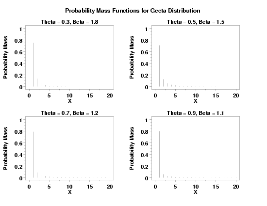
        
    plot generated by sample program

Program 2:
     
    SET GEETA DEFINITION MU
    LET MU   = 4.2
    LET BETA = 2.2
    LET Y = GEETA RANDOM NUMBERS FOR I = 1 1 500
    .
    LET Y3 XLOW XHIGH = INTEGER FREQUENCY TABLE Y
    CLASS LOWER 0.5
    CLASS WIDTH 1
    LET AMAX = MAXIMUM Y
    LET AMAX2 = AMAX + 0.5
    CLASS UPPER AMAX2
    LET Y2 X2 = BINNED Y
    .
    GEETA MLE Y
    RELATIVE HISTOGRAM Y2 X2
    LIMITS FREEZE
    PRE-ERASE OFF
    LINE COLOR BLUE
    PLOT GETPDF(X,MUML,BETAML) FOR X = 1  1  AMAX
    LIMITS
    PRE-ERASE ON
    LINE COLOR BLACK
    LET MU    = MUML
    LET BETA  = BETAML
    GEETA CHI-SQUARE GOODNESS OF FIT Y3 XLOW XHIGH
    CASE ASIS
    JUSTIFICATION CENTER
    MOVE 50 97
    TEXT Mu = ^MUML, Beta = ^BETAML
    MOVE 50 93
    TEXT Minimum Chi-Square = ^STATVAL, 95% CV = ^CUTUPP95
    .
    LABEL CASE ASIS
    X1LABEL Mu
    Y1LABLE Minimum Chi-Square
    GEETA KS PLOT Y3 XLOW XHIGH
    LET MU    = SHAPE1
    LET BETA  = SHAPE2
    GEETA CHI-SQUARE GOODNESS OF FIT Y3 XLOW XHIGH
    JUSTIFICATION CENTER
    MOVE 50 97
    TEXT Mu = ^MU, Beta = ^Beta
    MOVE 50 93
    TEXT Minimum Chi-Square = ^MINKS, 95% CV = ^CUTUPP95
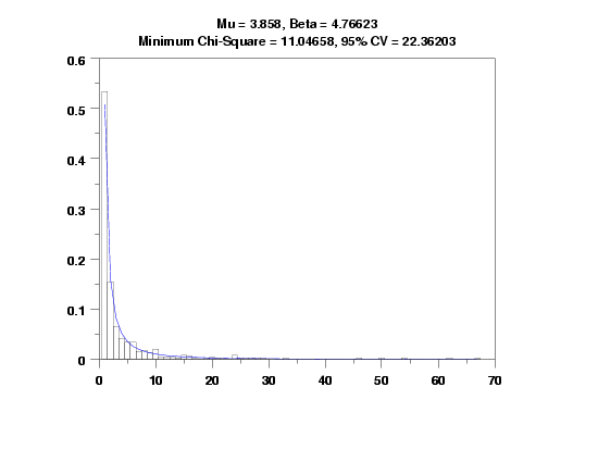
        
    plot generated by sample program
                       CHI-SQUARED GOODNESS-OF-FIT TEST
      
     NULL HYPOTHESIS H0:      DISTRIBUTION FITS THE DATA
     ALTERNATE HYPOTHESIS HA: DISTRIBUTION DOES NOT FIT THE DATA
     DISTRIBUTION:            GEETA
      
     SAMPLE:
        NUMBER OF OBSERVATIONS      =      500
        NUMBER OF NON-EMPTY CELLS   =       16
        NUMBER OF PARAMETERS USED   =        2
      
     TEST:
     CHI-SQUARED TEST STATISTIC     =    11.04658
        DEGREES OF FREEDOM          =       13
        CHI-SQUARED CDF VALUE       =    0.393085
      
        ALPHA LEVEL         CUTOFF              CONCLUSION
                10%       19.81193               ACCEPT H0
                 5%       22.36203               ACCEPT H0
                 1%       27.68825               ACCEPT H0
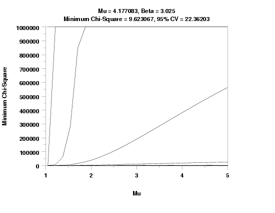
        
    plot generated by sample program
                       CHI-SQUARED GOODNESS-OF-FIT TEST
      
     NULL HYPOTHESIS H0:      DISTRIBUTION FITS THE DATA
     ALTERNATE HYPOTHESIS HA: DISTRIBUTION DOES NOT FIT THE DATA
     DISTRIBUTION:            GEETA
      
     SAMPLE:
        NUMBER OF OBSERVATIONS      =      500
        NUMBER OF NON-EMPTY CELLS   =       16
        NUMBER OF PARAMETERS USED   =        2
      
     TEST:
     CHI-SQUARED TEST STATISTIC     =    9.623067
        DEGREES OF FREEDOM          =       13
        CHI-SQUARED CDF VALUE       =    0.275571
      
        ALPHA LEVEL         CUTOFF              CONCLUSION
                10%       19.81193               ACCEPT H0
                 5%       22.36203               ACCEPT H0
                 1%       27.68825               ACCEPT H0
        

Date created: 8/23/2006
Last updated: 8/23/2006
Please email comments on this WWW page to alan.heckert@nist.gov.