CLUSTER

K MEANS CLUSTER
NORMAL MIXTURE CLUSTER
K MEDOIDS CLUSTER
FUZZY CLUSTER
AGNES CLUSTER
DIANA CLUSTER

Analysis Command

Perform a cluster analysis.

The goal of cluster analysis is to find groups in data. There are many approaches to this task. We can divide this into two primary approaches.
1. Partitioning Methods

   Given p variables each with n observations, we create k clusters and assign each of the n observations to one of these clusters.

   For these methods, the number of clusters typically has to be specified in advance. In Dataplot, to specify the number of clusters, enter the command

   LET NCLUSTER = <value>

   It is typical to run the cluster analysis for several different values of NCLUSTER.

   Dataplot implements the following partition based methods.

   • K-MEANS

     K-means is the workhorse method for clustering. The k-means critierion is to minimize the within cluster sum of squares based on Euclidean distances between the observations. That is, minimize

     \( \sum_{i=1}^{k}{W(C_{k})} = \sum_{i=1}^{k}{\sum_{x_{i} \in C_{k}} {(x_{i} - \mu_{k})^{2}}} \)

     with \( C_{k} \), \( x_{i} \), and \( \mu_{k} \) denoting the k-th cluster, an observation belonging to cluster k, and the mean value of the observations belonging to \( C_{k} \), respectively.

     Dataplot implements k- means using the Hartigan-Wong algorithm. This algorithm finds a local minimum, so different results can be obtained based on the initial assignment to clusters. The first method is to randomly select observations to use as initial cluster centers. The second method is suggested by Hartigan and Wong. First order the observations by their distances to the overall mean. Then for cluster L (L = 1, 2, ... k), use row \( 1 + (L-1) [\frac{p}{k}] \) as the initial cluster center.

     To specify the initialization method, enter

     SET K MEANS INITIAL

     The default is RANDOM.

   • K-MEDOIDS

     The k-medoids method was proposed by Kaufman and Rousseeuw. In k-medoids clustering, each cluster is represented by one observation in the cluster. These observations are called the cluster medoids. The cluster medoids correspond to the most centrally located observations in the cluster. The k-medoids method is more robust to outliers and noise than the k-means method. The mathematical details of the method are given in the Kaufman and Rousseeuw book (see References below).

     The k-medoids method can start either with the original measurement data or a distance matrix (this matrix will have dimension nxn).

     Kaufman and Rousseeuw provided two algorithms for k-medoid clustering.

     Partioning around medoids (PAM) is used when the number of observations is small (up to 100 observations in the original Kaufman and Rousseeuw code). All of the observations are used to determine the clusters.

     When the number of observations is larger, the CLARA algorithm is used. In CLARA, a number of random samples of the full data set are generated and the PAM algorithm is applied to them. The random sample that generates the best clustering is used to assign the unsampled observations to a cluster.

     In Dataplot, you can specify the cut-off between switching from PAM to CLARA with the command

     SET K MEDOID CLUSTER PAM MAXIMUM SIZE

     where <value> is between 100 and 500.

     You can also specify the number of samples drawn and the sample size for each sample with the commands

     SET K MEDOID CLUSTER NUMBER OF SAMPLES <value>
     SET K MEDOID CLUSTER NUMBER OF SAMPLES <value>
     

     The default is to draw 5 samples with 40 + 2*(number of clusters) observations per sample. For most applications, these defaults should be sufficient.

     The PAM and CLARA algorithms can be based on either Euclidean distances or Manhattan (city block) distances. To specify which to use, enter

     SET K MEDOID CLUSTER DISTANCE <EUCLIDEAN/MANHATTAN>
     

     The default is to use euclidean distances.

     Dataplot assumes if the number of rows and columns are equal that a distance matrix is being input. In the unlikely case where the they are equal for measurement data, you can enter the command

     SET K MEDOID CLUSTER TYPE MEASUREMENT

     To restore the default, enter

     SET K MEDOID CLUSTER TYPE DISSIMILARITY

     For the random sampling, Dataplot uses its own random number generator routines by default. You can request the genrator used by Kaufman and Rousseeuw by entering the command (this option is intended primarily to allow validating the Dataplot results against the results given by running the Kaufman and Rousseeuw codes directly)

     SET K MEDOID CLUSTER RANDOM NUMBER GENERATOR ROUSSEEUW

     To reset the default, enter

     SET K MEDOID CLUSTER RANDOM NUMBER GENERATOR DATAPLOT

     You can request that only the final results be printed by entering the command

     SET K MEDOID CLUSTER PRINT FINAL

     To rese the default where results for the individual samples are printed, enter

     SET K MEDOID CLUSTER PRINT ALL

   • FUZZY CLUSTERING (FANNY)

     Partioning algorithms typically assign each observation to a single cluster. Fuzzy clustering assigns each observation to every cluster with a probability for being in that cluster. Kaufman and Rousseeuw provide an algorithm, FANNY, to generate a fuzzy clustering. The details for FANNY are given in the Kaufman and Rousseeuw book.

     The following commands can be used with fanny clustering.

     SET FANNY CLUSTER DISTANCE <EUCLIDEAN/MANHATTAN>
     SET FANNY CLUSTER PRINT <ALL/FINAL>
     SET FANNY CLUSTER TYPE <MEASUREMENT/DISSIMILARITY>
     SET FANNY CLUSTER MAXIMUM SIZE <value>
     

     These options are similar to the options for k-medoids clustering. As with PAM, a maximum of 500 observations can be set.

     The primary advantage of this approach is that it gives some indication of the uncertainty of the cluster assignments. The algorithm does return the "most likely" cluster assignment which can be used in visualizing the results of the cluster analysis. The drawback is that interpretion can become difficult as the number of observations increases.

   • NORMAL MIXTURES

     This implements Hartigan's MIX algorithm. This is similar to FANNY in that it assigns probabilities for the cluster assignments. This method is based on the model that the observations is selected at random from one of k (where k is the number of clusters) multivariate normal populations. The mathematical details are given in Hartigan's book.

2. Hierchial Clustering

   Hierchial clustering typically starts with a distance or dissimilarity matrix.

   Hierchial clustering can be divided into agglomerative algorithms and divisive algorithms.

   With agglomerative algorithms, we start with each object in a separate cluster. Then at each step, the two "closest" clusters are merged. This process is repeated until all objects are in a single cluster.

   Divisive algorithms work in the opposite direction. That is, it starts with all objects in a single cluster. Then at each step, a cluster is split into two clusters. This is repeated until all objects are in their own cluster.

   • AGGLOMERATIVE NESTING (AGNES)

     Dataplot implements the AGNES algorithm given in the Kaufman and Rousseeuw book.

     The AGNES algorithm can start either with measurement data (i.e., p variables with n observations) or with a previously created dissimilarity matrix. For measurement data, the first step is to create a dissimilarity matrix. You can request that either Euclidean distances or Manhattan distances be used to create the dissimilarity matrix. To specify which distance measure to use, enter the command

     SET AGNES CLUSTER DISTANCE <EUCLIDEAN/MANHATTAN>

     The default is to use the Manhattan distance. If you want to use some other distance metric, see the Note section below which describes the use of the GENERATE MATRIX command with a number of different distance metrics.

     The link function defines the critierion that will be used to decide which two clusters are "closest" and will therefore be joined at each step. The supported link functions are

     • Average Linkage - The distance between two clusters, A and B, is defined as the average distance between the elements in cluster A and the elements in cluster B.

       This is the recommended choice of Kaufman and Rousseeuw and is the default used by Dataplot.

     • Complete Linkage - The distance between two clusters, A and B, is defined as the maximum distance of all pairwise distances between the elements in cluster A and the elements in cluster B.

     • Single Linkage - The distance between two clusters, A and B, is defined as the minimum distance of all pairwise distances between the elements in cluster A and the elements in cluster B. Single linkage clustering is also referred to as "nearest neighbor" clustering.

     • Centroid Linkage - The distance between two clusters, A and B, is defined as the distance between the centroid for cluster A and the centroid for cluster B.

       This method should be restricted to the case where the dissimilarity matrix is defined by Euclidean distances. Another drawback is that the dissimilarities between clusters are no longer monotone which makes visualizing the results problematic. For these reasons, average linkage is typically preferred to centroid linkage.

     • Ward's Linkage - This method minimizes the total within-cluster variance. At each step, the pair of clusters with minimum between-cluster distance are merged.

       As with centroid linkage, Ward's linkage is intended for the case where Euclidean distances are used. According to Kaufman and Rousseeuw, this method only performs well if an approximately equal number of objects is drawn from each population and it has problems with clusters of unequal diameter. Also, it may have problems when the clusters are ellipsoidal (i.e., variables are correlated within clusters) rather than spherical.

     • Weighted Average Linkage - This method is a variant of average linkage. This method was proposed by Sokal and Sneath. See Kaufman and Rousseeuw for details.

     • Gower's Linkage - This is a variant of the centroid method and should also be restricted to the case of Euclidean distances. See Kaufman and Rousseeus for details.

     In practice, average linkage, complete linkage, and single linkage are the methods most commonly used. Kaufman and Rousseeuw review the properties of various linkage methods and reference several other studies. In summary, although no method is best in all cases, they find that average linkage typically performs well in practice and is reasonably robust to slight distortions. Studies they cite indicate that single linkage, although easy to implement and understand, typically does not perform as well as average linkage or complete linkage.

     To specify the linkage method to use, enter one of the following commands

     SET AGNES CLUSTER METHOD AVERAGE LINKAGE
     SET AGNES CLUSTER METHOD COMPLETE LINKAGE
     SET AGNES CLUSTER METHOD SINGLE LINKAGE
     SET AGNES CLUSTER METHOD WEIGHTED AVERAGE ...
                 LINKAGE
     SET AGNES CLUSTER METHOD WARD
     SET AGNES CLUSTER METHOD CENTROID
     SET AGNES CLUSTER METHOD GOWER
     

     You can specify the maximum number of rows/columns in the distance matrix (if you start with measurement data, this is the number of columns) with the command

     SET AGNES CLUSTER MAXIMUM SIZE <value>

     where <value> is between 100 and 500 (the default is 100).

     You can control the amount of output generated by agnes clustering with the command

     SET AGNES CLUSTER PRINT <ALL/FINAL>

     Using FINAL omits the printing of the distance matrix.

     Dataplot assumes if the number of rows and columns are equal that a distance matrix is being input. In the unlikely case where the they are equal for measurement data, you can enter the command

     SET AGNES CLUSTER TYPE MEASUREMENT

     To restore the default, enter

     SET AGNES CLUSTER TYPE DISSIMILARITY

   • DIVISIVE (DIANA)

     Dataplot implements the DIANA algorithm given in the Kaufman and Rousseeuw book. The details of the algorithm are given there. DIANA is currently limited to using average distances between clusters.

     The options used for agnes clustering also apply to diana clustering. The exception is that diana only supports the average linkage method.

The traditional clustering methods described above are heuristic methods and are intented for small to moderate size data sets. These methods tend to work reasonably well for spherical shaped or convex clusters. If clusters are not compact and well separated, these methods may not be effective. The k-means algorithm is sensitive to noise and outliers (the k-medoids method may work better in these cases).

Dataplot does not currently support model-based clustering or some of the newer cluster methods such as DBSCAN that can work better for non-spherical shapes in the presence of significant noise.

K MEANS CLUSTER <y1> ... <yk>
                        <SUBSET/EXCEPT/FOR qualification>
where <y1> ... <yk> is a list of response variables;
and where the <SUBSET/EXCEPT/FOR qualification> is optional.

This syntax performs Hartigan's k-means clustering.

NORMAL MIXTURE CLUSTER <y1> ... <yk>
                        <SUBSET/EXCEPT/FOR qualification>
where <y1> ... <yk> is a list of response variables;
and where the <SUBSET/EXCEPT/FOR qualification> is optional.

This syntax performs Hartigan's normal mixture clustering.

K MEDIODS CLUSTER <y1> ... <yk>
                        <SUBSET/EXCEPT/FOR qualification>
where <y1> ... <yk> is a list of response variables;
and where the <SUBSET/EXCEPT/FOR qualification> is optional.

This syntax performs Kaufman and Rousseeuw k-medoids clustering. The use of PAM or CLARA will be determined based on the number of objects to be clustered.

FANNY CLUSTER <y1> ... <yk>
                        <SUBSET/EXCEPT/FOR qualification>
where <y1> ... <yk> is a list of response variables;
and where the <SUBSET/EXCEPT/FOR qualification> is optional.

This syntax performs Kaufman and Rousseeuw fuzzy clustering using the FANNY algorithm.

AGNES CLUSTER <y1> ... <yk>
                        <SUBSET/EXCEPT/FOR qualification>
where <y1> ... <yk> is a list of response variables;
and where the <SUBSET/EXCEPT/FOR qualification> is optional.

This syntax performs Kaufman and Rousseeuw agglomerative nesting clustering using the AGNES algorithm.

By default, this algoritm uses the average distance linking critierion. However, it can also be used for single linkage (nearest neighbor), complete linkage, Ward's method, the centroid method, and Gower's method. See above for details.

DIANA CLUSTER <y1> ... <yk>
                        <SUBSET/EXCEPT/FOR qualification>
where <y1> ... <yk> is a list of response variables;
and where the <SUBSET/EXCEPT/FOR qualification> is optional.

This syntax performs Kaufman and Rousseeuw divisive clustering using the DIANA algorithm.

K MEANS CLUSTERING Y1 Y2 Y3 Y4 Y5 Y6
K MEANS CLUSTERING Y1 TO Y6
K MEDOIDS CLUSTERING Y1 TO Y6
AGNES CLUSTERING M

When starting with measurement data, if the variables being clustered use different measurement scales, it may be desirable to standardize the data before applying the clustering algorithm. Standardization creates unitless variables.

The desirability of standardization will depend on the specific data set. Kaufman and Rousseeuw (pp. 8-11) discuss some of the issues in deciding whether or not to standardize. By default, Dataplot will standardize the variables.

The following commands can be used to specify whether or not you want the variables to be standardized

SET K MEANS SCALE <ON/OFF>
SET NORMAL MIXTURE SCALE <ON/OFF>
SET K MEDOIDS SCALE <ON/OFF>
SET FANNY SCALE <ON/OFF>
SET AGNES SCALE <ON/OFF>


The SET AGNES SCALE command also applies to the DIANA CLUSTER command.

If you choose to standardize, the basic formula is

\( Y_{i} = \frac{X_{i} - loc}{scale} \)

where loc and scale denote the desired location and scale parameters.

To specify the location statistic, enter

SET LOCATION STATISTIC <stat>

where <stat> is one of: MEAN, MEDIAN, MIDMEAN. HARMONIC MEAN, GEOMETRIC MEAN, BIWEIGHT LOCATION, H10, H12, H15, H17, or H20.

To specify the scale statistic, enter

SET SCALE STATISTIC <stat>

where <stat> is one of: STANDARD DEVIATION, H10, H12, H15, H17, H20, BIWEIGHT SCALE, MEDIAN ABSOLUTE DEVIATION, SCALED MEDIAN ABSOLUTE DEVIATION, AVERAGE ABSOLUTE DEVIATION, INTERQUARTILE RANGE, NORMALIZED INTERQUARTILE RANGE, SN SCALE, or RANGE.

The default is to use the mean for the location statistic and the standard deviation for the scale statistic. Rousseeuw recommends using the mean for the location statistic and the average absolute deviation for the scale statistic.

Several of the clustering algorithms can start with a distance matrix. Dataplot offers a number of commands for converting measurement data to distances or dissimilarities. Note that the GENERATE MATRIX command can be used to convert measurement data to a distance matrix for a specified statistic. For example,
LET M = GENERATE MATRIX COSINE DISTANCE X1 X2 X3 X4

The COSINE DISTANCE can be replaced with a number of other distance measures.

1. For continuous data, the following distance measures are supported

   EUCLIDEAN DISTANCE	-	Euclidean distance
   MANHATTAN DISTANCE	-	Manhattan (city block) distance
   MINKOWSKI DISTANCE	-	Minkowski distance
   CHEBYCHEV DISTANCE	-	Chebyshev distance
   COSINE DISTANCE	-	cosine distance
   ANGULAR COSINE DISTANCE	-	angular cosine distance

2. For binary data, a number of distance measures are available. Enter HELP BINARY MATCH DISSIMILARITIES for details.

3. For correlation type measures (often used when clustering variables rather than observations), the following are supported

   PEARSON DISSIMILARITY	-	\( \frac{1 - r}{2} \) where \( r \) is the Pearson correlation coefficient
   SPEARMAN DISSIMILARITY	-	\( \frac{1 - r}{2} \) where \( r \) is the Spearman rank correlation coefficient
   KENDALL TAU DISSIMILARITY	-	\( \frac{1 - r}{2} \) where \( r \) is the Kendall tau correlation coefficient

One issue with clustering is how to visualize the results. The Dataplot clustering commands do not generate any graphics directly. Instead, Dataplot writes information to files that allow several different approaches to visualization. Different graphical approaches are typically used for partitioning and hierchial methods, so we will discuss these separately.
1. Partion Methods
   • Dataplot writes the cluster id for each observation to the file dpst1f.dat. So one visualization approach is to generate a scatter plot matrix of the variables and use the cluster id to identify the different clusters in the plots. This is demonstrated in the Program 1 and 2 examples below.

   • Another approach is to plot the first two principal components. Again, the cluster id can be used to identify the clusters. This is demonstrated in the Program 1 and 2 examples below.

   • Rousseeuw advocated the silhouette plot. For each observation, compute
     \( s_{i} = \frac{b_{i} - a_{i}} {\max(a_{i},b_{i})} \)

     where

     \( a_{i} \)	=	the average dissimilarity of the i-th point with all other points in the cluster to which it belongs
     \( b_{i} \)	=	the lowest average dissimilarity of the i-th point with all other clusters. The \( b_{i} \) value can be considered the second best choice for observation i.

     The \( s_{i} \) values will be between -1 and 1. A value near 0 indicates that \( a_{i} \) and \( b_{i} \) are nearly equal and thus indicating the choice between assigning object i to A or B is ambiguous. On the other hand, when \( s_{i} \) is close to 1, this indicates that the within dissimilarity is much smaller than the smallest between dissimilarity. This indicates good clustering. Negative values of \( s_{i} \) indicate that B may in fact be a better choice than A, so the observation may be misclassified.

     The average \( s_{i} \) for each cluster and the average \( s_{i} \) for all observations can be computed. These provide a measure of the quality of the clustering. In particular, they can be used to pick appropriate number of clusters to use (i.e., the number of clusters which results in the highest average for all the \( s_{i} \) values).

     Dataplot writes the \( s_{i} \) values (with the cluser id values) to dpst4f.dat. This is demonstrated in the Program 1, 2 and 3 examples below.

2. Hierchial Methods
   • Kaufman and Rousseeuw provide a line printer "banner" plot for their AGNES and DIANA algorithms. To include this plot in the clustering output, enter the command

     SET AGNES CLUSTERING BANNER PLOT ON

     The default is OFF.

   • The most commonly used visualization technique for hierchial clustering is the dendogram. Dataplot writes the plot coordinates for the dendogram to dpst3f.dat. The ordering of the clusters is written to dpst1f.dat. Program examples 4 and 5 demonstrate how to plot the dendogram from the information in these files. The Program 4 example generates a horizontal dendogram and the Program 5 example generates a vertical dendogram.

     The dendogram is basically a variant of a tree diagram. It shows the order the clusters were joined as well as the distance between clusters. One axis contains the objects to be clustered in a sorted order while the other axis is distance. The dendogram shows which clusters were connected at each step and shows the distance between these clusters.

   • Another popular technique is the icicle plot introduced by Kruskal and Landwehr (1983). Although the original article introduced this as a line printer graphic, it can be adapted for modern graphical displays. The Program 4 and Program 5 examples demonstrate how to generate an icicle plot from the information written to files dpst1f.dat and dpst2f.dat.

     Many different variants of the icicle plot are shown in the literature. But the basic idea is that one axis contains the number of clusters while the other axis shows the objects being clustered. For each object, two rows (or columns) are drawn (the last object only has a single row). The coordinate for one row (or column) shows where the object joined the cluster from one direction (i.e., top or left) while the coordinate for the second row (or column) shows where the object joined the cluster from the other direction. If you scan down the "number of cluster" axis, contiguous rows (or columns) indicate objects that belong to the same cluster. Note that the icicle plot does not give any indication of the distance. The banner plot of Kaufman and Rousseeuw is similar to the icicle plot although they do show distances (on a 0 to 100 percentage scale rather than in raw distance units).

     The Program examples below show the icicle plots as simple bar graphs that are read from left to right (or bottom to top). Variants of the icicle plot often show these as rows (or columns) of asterisks or use a right to left (or top to bottom) orientation. These variants are a matter of taste and can be generated from the information written to files dpst1f.dat and dpst2f.dat.

None

K MEANS is a synonym for K MEANS CLUSTER
K MEDOIDS is a synonym for K MEDOIDS CLUSTER
FANNY is a synonym for FANNY CLUSTER
AGNES is a synonym for AGNES CLUSTER
DIANA is a synonym for DIANA CLUSTER

PEARSON DISSIMILARITY	=	Compute the dissimilarity of two variables based on Pearson correlation.
SPEARMAN DISSIMILARITY	=	Compute the dissimilarity of two variables based on Spearman's rank correlation.
KENDALL TAU DISSIMILARITY	=	Compute the dissimilarity of two variables based on Kendall's tau correlation.
COSINE DISTANCE	=	Compute the cosine distance.
MANHATTAN DISTANCE	=	Compute the Euclidean distance.
EUCLIDEAN DISTANCE	=	Compute the Euclidean distance.
MATRIX DISTANCE	=	Compute various distance metrics for a matrix.
GENERATE MATRIX <stat>	=	Compute a matrix of pairwise statistic values.

Hartigan and Wong (1979), "Algorithm AS 136: A K-Means Clustering Algorithm", Applied Statistics, Vol. 28, No. 1.

Hartigan (1975), "Clustering Algorithms", Wiley.

Kaufman and Rousseeuw (1990), "Finding Groups in Data: An Introduction To Cluster Analysis", Wiley.

Rousseeuw (1987), "Silhouettes: A Graphical Aid to the Interpretation and Validation of Cluster Analysis", Journal of Computational and Applied Mathematics, North Holland, Vol. 20, pp. 53-65.

Kruskal and Landwehr (1983), "Icicle Plots: Better Displays for Hierarchial Clustering", The American Statistician, Vol. 37, No. 2, pp. 168.

Multivariate Analysis, Exploratory Data Analysis

2017/09
2017/11: Changed the default for standardization to be ON
                 rather than OFF. Fixed a bug where the k-means
                 method always performed standardization. For
                 k-means, the cluster centers written to dpst3f.dat
                 were modified to write the unstandardized values
                 rather than the standardized values.

 
case asis
label case asis
title case asis
title offset 2
.
. Step 1:   Read the data
.
dimension 100 columns
skip 25
read iris.dat y1 y2 y3 y4 x
skip 0
set write decimals 3
.
. Step 2:   Perform the k-means cluster analysis with 3 clusters
.
set random number generator fibbonacci congruential
seed 45617
let ncluster = 3
set k means initial distance
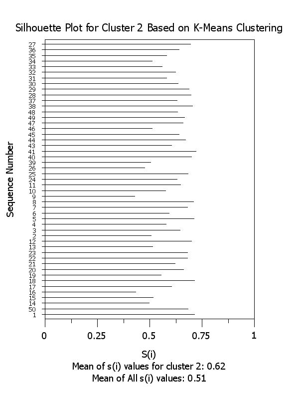
set k means silhouette on
feedback off
k-means y1 y2 y3 y4
    

The following output is generated

            Summary of K-Means Cluster Analysis
 
---------------------------------------------
                     Number            Within
                  of Points           Cluster
     Cluster     in Cluster    Sum of Squares
---------------------------------------------
           1             53            64.496
           2             49            39.774
           3             48            53.736
    

read dpst4f.dat clustid si
.
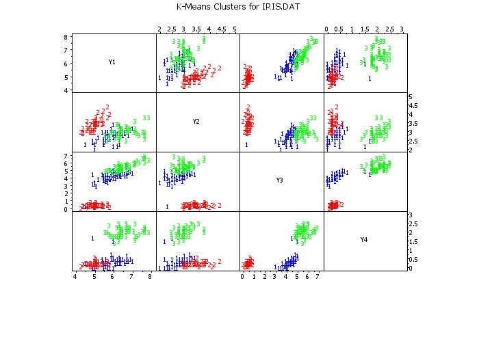
. Step 3:   Scatter plot matrix with clusters identified
.
line blank all
char 1 2 3
char color blue red green
frame corner coordinates 5 5 95 95
multiplot scale factor 4
tic offset units screen
tic offset 5 5
.
set scatter plot matrix tag on
scatter plot matrix y1 y2 y3 y4 clustid
.
justification center
move 50 97
text K-Means Clusters for IRIS.DAT
    



.
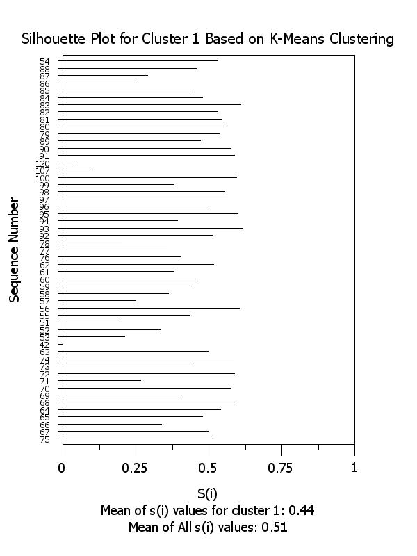
. Step 4:   Silhouette Plot
.
.           For better resolution, show the results for
.           each cluster separately
.
let ntemp = size clustid
let indx = sequence 1 1 ntemp
let clustid = sortc clustid si indx
let x = sequence 1 1 ntemp
loop for k = 1 1 ntemp
    let itemp = indx(k)
    let string t^k = ^itemp
end of loop
.
orientation portrait
device 2 color on
frame corner coordinates 15 20 85 90
tic offset units data
horizontal switch on
.
spike on
char blank all
line blank all
.
label size 1.7
xlimits 0 1
xtic mark offset 0 0
x1label S(i)
x1tic mark label size 1.7
y1tic mark offset 0.8 0.8
minor y1tic mark number 0
y1tic mark label format group label
y1tic mark label size 1.2
y1tic mark size 0.8
y1label Sequence Number
.
let simean  = mean si
let simean  = round(simean,2)
x3label Mean of All s(i) values: ^simean
.
loop for k = 1 1 ncluster
    let sit = si
    let xt  = x
    retain sit xt subset clustid = k
    let ntemp2 = size sit
    let y1min = minimum xt
    let y1max = maximum xt
    y1limits y1min y1max
    major y1tic mark number ntemp2
    let ig = group label t^y1min to t^y1max
    y1tic mark label content ig
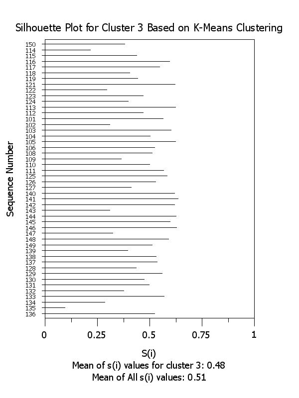
    title Silhouette Plot for Cluster ^k Based on K-Means Clustering
    .
    let simean^k = mean si subset clustid = k
    let simean^k = round(simean^k,2)
    x2label Mean of s(i) values for cluster ^k: ^simean^k
    .
    plot si x subset clustid = k
end of loop
.
label
ylimits
major y1tic mark number
minor y1tic mark number
y1tic mark label format numeric
y1tic mark label content
y1tic mark label size
    







.
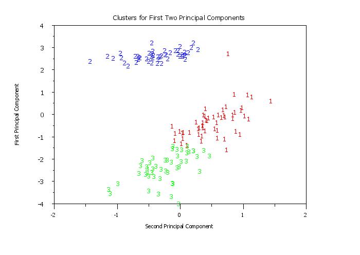
. Step 5:   Display clusters in terms of first 2 principal components
.
orientation landscape
.
let ym = create matrix y1 y2 y3 y4
let pc = principal components ym
read dpst1f.dat clustid
spike blank all
character 1 2 3
character color red blue green
horizontal switch off
tic mark offset 0 0
limits
title Clusters for First Two Principal Components
y1label First Principal Component
x1label Second Principal Component
x2label
.
plot pc1 pc2 clustid
    

 
case asis
label case asis
title case asis
title offset 2
.
. Step 1:   Read the data
.
dimension 100 columns
skip 25
read iris.dat y1 y2 y3 y4 x
skip 0
set write decimals 3
.
. Step 2:   Perform the k-medoids cluster analysis with 3 clusters
.
set random number generator fibbonacci congruential
seed 45617
let ncluster = 3
set k medoids cluster distance manhattan
k medoids y1 y2 y3 y4
    

The following output is generated

           **********************************************
           *                                            *
           *  ROUSSEEUW/KAUFFMAN K-MEDOID CLUSTERING    *
           *  (USING THE CLARA ROUTINE).                *
           *                                            *
           **********************************************
  
  
 **********************************************
 *                                            *
 *  NUMBER OF REPRESENTATIVE OBJECTS     3    *
 *                                            *
 **********************************************
  
    5 SAMPLES OF    46 OBJECTS WILL NOW BE DRAWN.
  
 SAMPLE NUMBER    1
 ******************
  
 RANDOM SAMPLE =
            2      4      8      9     14     16     19     23     26     27
           30     32     37     38     39     40     43     44     45     46
           49     50     52     53     54     57     62     64     72     87
           89     94     97    102    104    106    109    117    127    130
          135    141    142    143    147    148
  
 RESULT OF BUILD FOR THIS SAMPLE
   AVERAGE DISTANCE =       1.00870
  
 FINAL RESULT FOR THIS SAMPLE
   AVERAGE DISTANCE  =          0.978
  
 RESULTS FOR THE ENTIRE DATA SET
   TOTAL DISTANCE    =         174.900
   AVERAGE DISTANCE  =           1.166
  
   CLUSTER SIZE MEDOID    COORDINATES OF MEDOID
  
         1   50      8         5.00       3.40       0.50       0.20
  
         2   51     62         5.90       3.00       4.20       0.50
  
         3   49    117         6.50       3.00       5.50       1.80
  
   AVERAGE DISTANCE TO EACH MEDOID
          0.75       1.34
  
   MAXIMUM DISTANCE TO EACH MEDOID
          1.90       3.10
   MAXIMUM DISTANCE TO A MEDOID DIVIDED BY MINIMUM
   DISTANCE OF THE MEDOID TO ANOTHER MEDOID
          0.36       0.97
  
 SAMPLE NUMBER    2
 ******************
  
 RANDOM SAMPLE =
            2      8     20     22     24     27     30     32     34     35
           36     37     39     40     43     49     50     52     56     61
           62     63     65     66     71     72     73     74     83     86
           95     97     98    101    117    118    121    126    132    133
          140    141    143    144    146    150
  
 RESULT OF BUILD FOR THIS SAMPLE
   AVERAGE DISTANCE =       0.97174
  
 FINAL RESULT FOR THIS SAMPLE
   AVERAGE DISTANCE  =          0.970
  
 RESULTS FOR THE ENTIRE DATA SET
   TOTAL DISTANCE    =         181.100
   AVERAGE DISTANCE  =           1.207
  
   CLUSTER SIZE MEDOID    COORDINATES OF MEDOID
  
         1   50      8         5.00       3.40       0.50       0.20
  
         2   55     97         5.70       2.90       4.20       0.30
  
         3   45    121         6.90       3.20       5.70       2.30
  
   AVERAGE DISTANCE TO EACH MEDOID
          0.75       1.38
  
   MAXIMUM DISTANCE TO EACH MEDOID
          1.90       3.00
   MAXIMUM DISTANCE TO A MEDOID DIVIDED BY MINIMUM
   DISTANCE OF THE MEDOID TO ANOTHER MEDOID
          0.38       0.60
  
 SAMPLE NUMBER    3
 ******************
  
 RANDOM SAMPLE =
            8     12     13     15     22     23     24     25     26     27
           32     33     35     39     40     43     44     46     47     49
           52     58     59     62     63     67     72     75     80     86
           97     99    100    110    113    115    117    119    123    125
          137    139    143    145    148    149
  
 RESULT OF BUILD FOR THIS SAMPLE
   AVERAGE DISTANCE =       1.01522
  
 FINAL RESULT FOR THIS SAMPLE
   AVERAGE DISTANCE  =          1.015
  
 RESULTS FOR THE ENTIRE DATA SET
   TOTAL DISTANCE    =         171.100
   AVERAGE DISTANCE  =           1.141
  
   CLUSTER SIZE MEDOID    COORDINATES OF MEDOID
  
         1   50      8         5.00       3.40       0.50       0.20
  
         2   50     97         5.70       2.90       4.20       0.30
  
         3   50    113         6.80       3.00       5.50       2.10
  
   AVERAGE DISTANCE TO EACH MEDOID
          0.75       1.25
  
   MAXIMUM DISTANCE TO EACH MEDOID
          1.90       2.90
   MAXIMUM DISTANCE TO A MEDOID DIVIDED BY MINIMUM
   DISTANCE OF THE MEDOID TO ANOTHER MEDOID
          0.38       0.67
  
 SAMPLE NUMBER    4
 ******************
  
 RANDOM SAMPLE =
            4      5      6      8     11     12     15     20     23     26
           37     40     42     43     45     47     53     56     61     63
           68     72     73     90     93     97    103    104    105    108
          113    117    120    122    126    127    129    130    134    135
          138    140    143    144    149    150
  
 RESULT OF BUILD FOR THIS SAMPLE
   AVERAGE DISTANCE =       1.00435
  
 FINAL RESULT FOR THIS SAMPLE
   AVERAGE DISTANCE  =          0.983
  
 RESULTS FOR THE ENTIRE DATA SET
   TOTAL DISTANCE    =         177.100
   AVERAGE DISTANCE  =           1.181
  
   CLUSTER SIZE MEDOID    COORDINATES OF MEDOID
  
         1   50     40         5.10       3.40       0.50       0.20
  
         2   49     93         5.80       2.60       4.00       0.20
  
         3   51    117         6.50       3.00       5.50       1.80
  
   AVERAGE DISTANCE TO EACH MEDOID
          0.76       1.34
  
   MAXIMUM DISTANCE TO EACH MEDOID
          2.00       3.00
   MAXIMUM DISTANCE TO A MEDOID DIVIDED BY MINIMUM
   DISTANCE OF THE MEDOID TO ANOTHER MEDOID
          0.40       0.71
  
 SAMPLE NUMBER    5
 ******************
  
 RANDOM SAMPLE =
            8     12     16     17     18     23     24     26     29     41
           44     48     49     51     52     54     55     56     57     59
           62     66     67     71     73     77     79     81     97    100
          101    102    106    108    111    113    114    117    118    120
          121    123    127    134    137    146
  
 RESULT OF BUILD FOR THIS SAMPLE
   AVERAGE DISTANCE =       1.09130
  
 FINAL RESULT FOR THIS SAMPLE
   AVERAGE DISTANCE  =          1.091
  
 RESULTS FOR THE ENTIRE DATA SET
   TOTAL DISTANCE    =         172.800
   AVERAGE DISTANCE  =           1.152
  
   CLUSTER SIZE MEDOID    COORDINATES OF MEDOID
  
         1   50      8         5.00       3.40       0.50       0.20
  
         2   53     79         6.00       2.90       4.50       0.50
  
         3   47    113         6.80       3.00       5.50       2.10
  
   AVERAGE DISTANCE TO EACH MEDOID
          0.75       1.33
  
   MAXIMUM DISTANCE TO EACH MEDOID
          1.90       3.40
   MAXIMUM DISTANCE TO A MEDOID DIVIDED BY MINIMUM
   DISTANCE OF THE MEDOID TO ANOTHER MEDOID
          0.33       0.97
  
  
  
 FINAL RESULTS
 *************
  
 SAMPLE NUMBER   3 WAS SELECTED, WITH OBJECTS =
       8     12     13     15     22     23     24     25     26     27
      32     33     35     39     40     43     44     46     47     49
      52     58     59     62     63     67     72     75     80     86
      97     99    100    110    113    115    117    119    123    125
     137    139    143    145    148    149
  
    AVERAGE DISTANCE FOR THE ENTIRE DATA SET =        1.141
  
  
    CLUSTERING VECTOR
    *****************
  
       1  1  1  1  1  1  1  1  1  1  1  1  1  1  1  1  1  1  1  1  1  1  1  1  1
       1  1  1  1  1  1  1  1  1  1  1  1  1  1  1  1  1  1  1  1  1  1  1  1  1
       2  2  2  2  2  2  2  2  2  2  2  2  2  2  2  2  2  2  2  2  2  2  2  2  2
       2  2  3  2  2  2  2  2  2  2  2  2  2  2  2  2  2  2  2  2  2  2  2  2  2
       3  3  3  3  3  3  2  3  3  3  3  3  3  3  3  3  3  3  3  3  3  3  3  3  3
       3  3  3  3  3  3  3  3  3  3  3  3  3  3  3  3  3  3  3  3  3  3  3  3  3
  
  
     CLUSTER SIZE MEDOID OBJECTS
  
           1   50      8
                             1    2    3    4    5    6    7    8    9   10
                            11   12   13   14   15   16   17   18   19   20
                            21   22   23   24   25   26   27   28   29   30
                            31   32   33   34   35   36   37   38   39   40
                            41   42   43   44   45   46   47   48   49   50
  
           2   50     97
                            51   52   53   54   55   56   57   58   59   60
                            61   62   63   64   65   66   67   68   69   70
                            71   72   73   74   75   76   77   79   80   81
                            82   83   84   85   86   87   88   89   90   91
                            92   93   94   95   96   97   98   99  100  107
  
           3   50    113
                            78  101  102  103  104  105  106  108  109  110
                           111  112  113  114  115  116  117  118  119  120
                           121  122  123  124  125  126  127  128  129  130
                           131  132  133  134  135  136  137  138  139  140
                           141  142  143  144  145  146  147  148  149  150
  
  
     AVERAGE DISTANCE TO EACH MEDOID
          0.750       1.248       1.424
  
     MAXIMUM DISTANCE TO EACH MEDOID
          1.900       2.900       3.000
  
     MAXIMUM DISTANCE TO A MEDOID DIVIDED BY MINIMUM
          0.380       0.674       0.698
    

skip 1
read dpst4f.dat clustid si
skip 0
.
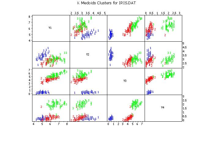
. Step 3:   Scatter plot matrix with clusters identified
.
line blank all
char 1 2 3
char color blue red green
frame corner coordinates 5 5 95 95
multiplot scale factor 4
tic offset units screen
tic offset 5 5
.
set scatter plot matrix tag on
scatter plot matrix y1 y2 y3 y4 clustid
.
justification center
move 50 97
text K Medoids Clusters for IRIS.DAT
    



.
. Step 4:   Silhouette Plot
.
.           For better resolution, show the results for
.           each cluster separately
.
let ntemp = size clustid
let indx = sequence 1 1 ntemp
let clustid = sortc clustid si indx
let x = sequence 1 1 ntemp
loop for k = 1 1 ntemp
    let itemp = indx(k)
    let string t^k = ^itemp
end of loop
.
orientation portrait
device 2 color on
frame corner coordinates 15 20 85 90
tic offset units data
horizontal switch on
.
spike on
char blank all
line blank all
.
label size 1.7
xlimits 0 1
xtic mark offset 0 0
x1label S(i)
x1tic mark label size 1.7
y1tic mark offset 0.8 0.8
minor y1tic mark number 0
y1tic mark label format group label
y1tic mark label size 1.2
y1tic mark size 0.8
y1label Sequence Number
.
let simean  = mean si
let simean  = round(simean,2)
x3label Mean of All s(i) values: ^simean
.
orientation portait
device 2 color on
loop for k = 1 1 ncluster
    .
    .
    let sit = si
    let xt  = x
    retain sit xt subset clustid = k
    let ntemp2 = size sit
    let y1min = minimum xt
    let y1max = maximum xt
    y1limits y1min y1max
    major y1tic mark number ntemp2
    let ig = group label t^y1min to t^y1max
    y1tic mark label content ig
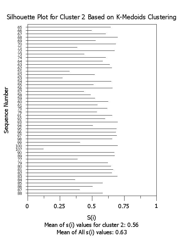
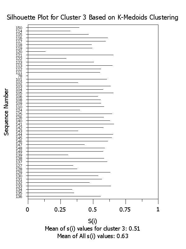
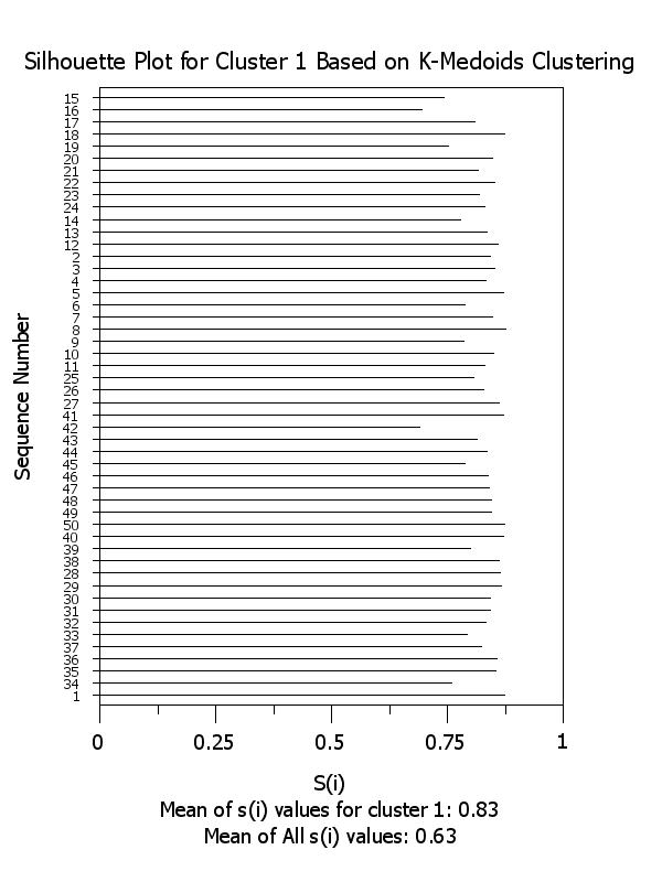
    title Silhouette Plot for Cluster ^k Based on K-Medoids Clustering
    .
    let simean^k = mean si subset clustid = k
    let simean^k = round(simean^k,2)
    x2label Mean of s(i) values for cluster ^k: ^simean^k
    .
    plot si x subset clustid = k
end of loop
.
label
ylimits
major y1tic mark number
minor y1tic mark number
y1tic mark label format numeric
y1tic mark label content
y1tic mark label size
    







.
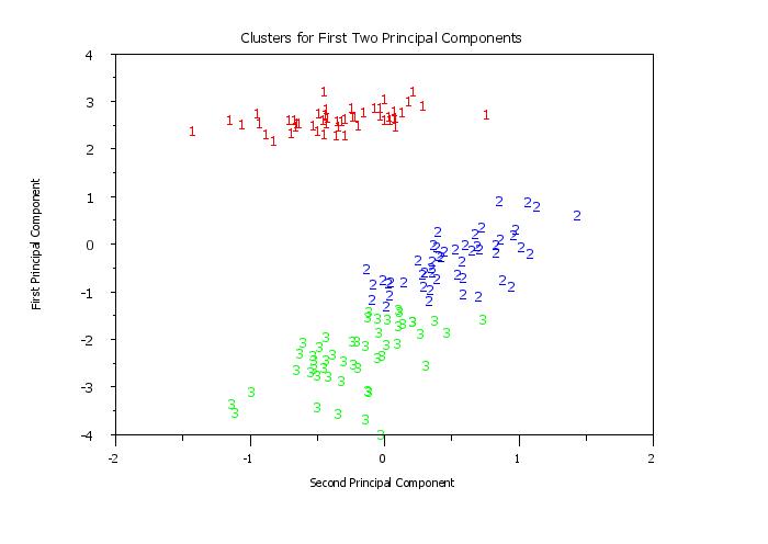
. Step 5:   Display clusters in terms of first 2 principal components
.
orientation landscape
device 2 color on
.
let ym = create matrix y1 y2 y3 y4
let pc = principal components ym
read dpst1f.dat clustid
spike blank all
character 1 2 3
character color red blue green
horizontal switch off
tic mark offset 0 0
limits
title Clusters for First Two Principal Components
y1label First Principal Component
x1label Second Principal Component
x2label
.
plot pc1 pc2 clustid
    

 
orientation portait
.
case asis
label case asis
title case asis
title offset 2
.
. Step 1:   Read the data
.
set write decimals 3
dimension 100 columns
.
skip 25
read matrix rouss1.dat y
skip 0
.
let string s1  = Belgium
let string s2  = Brazil
let string s3  = China
let string s4  = Cuba
let string s5  = Egypt
let string s6  = France
let string s7  = India
let string s8  = Israel
let string s9  = USA
let string s10 = USSR
let string s11 = Yugoslavia
let string s12 = Zaire
.
. Step 2:   Perform the k-mediods cluster analysis with 3 clusters
.
let ncluster = 3
.
capture screen on
capture CLUST4A.OUT
k medioids y
end of capture
skip 1
read dpst4f.dat indx clustid si neighbor
skip 0
.
. Step 3:   Silhouette Plot
.
.           Create axis label
.
.           First sort by cluster and then sort by
.           silhouette within cluster (this second step
.           is a bit convoluted)
.
let simean = mean si
let simean = round(simean,2)
.
let ntemp = size indx
let clustid = sortc clustid si indx neighbor
.
loop for k = 1 1 ncluster
    .
    let simean^k = mean si subset clustid = ^k
    let simean^k = round(simean^k,2)
    .
    let clustidt = clustid
    let sit = si
    let indxt = indx
    let neight = neighbor
    retain clustidt sit indxt neight subset clustid = k
    .
    let sit = sortc sit clustidt indxt neight
    if k = 1
       let clustid2 = clustidt
       let si2 = sit
       let indx2 = indxt
       let neigh2 = neight
    else
       let clustid2 = combine clustid2 clustidt
       let si2 = combine si2 sit
       let indx2 = combine indx2 indxt
       let neigh2 = combine neigh2 neight
    end of if
end of loop
let clustid = clustid2
let si = si2
let indx = indx2
let neighbor = neigh2
.
loop for k = 1 1 ntemp
    let itemp = indx(k)
    let string t^k = ^s^itemp
end of loop
let ig = group label t1 to t^ntemp
.
let x = sequence 1 1 ntemp
.
frame corner coordinates 15 20 85 90
tic offset units data
horizontal switch on
.
spike on all
spike color red blue green
char blank all
line blank all
.
xlimits 0 1
xtic mark offset 0 0
major xtic mark number 6
x1tic mark decimal 1
y1limits 1 ntemp
y1tic mark offset 1 1
major y1tic mark number ntemp
minor y1tic mark number 0
y1tic mark label format group label
y1tic mark label content ig
y1tic mark label size 1.1
y1tic mark size 0.1
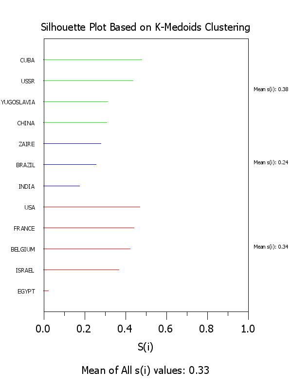
x1label S(i)
x3label Mean of All s(i) values: ^simean
title Silhouette Plot Based on K-Medoids Clustering
.
plot si x clustid
.
height 1.0
justification left
movesd 87 3
text Mean s(i): ^simean1
movesd 87 7
text Mean s(i): ^simean2
movesd 87 10.5
text Mean s(i): ^simean3
height 2
.
print indx clustid neighbor si
    

The following output is generated

 
           **********************************************
           *                                            *
           *  ROUSSEEUW/KAUFFMAN K-MEDOID CLUSTERING    *
           *  (USING THE PAM ROUTINE).                  *
           *                                            *
           **********************************************
  
  
  
 DISSIMILARITY MATRIX
 --------------------
    1
    2       5.58
    3       7.00     6.50
    4       7.08     7.00     3.83
    5       4.83     5.08     8.17     5.83
    6       2.17     5.75     6.67     6.92     4.92
    7       6.42     5.00     5.58     6.00     4.67     6.42
    8       3.42     5.50     6.42     6.42     5.00     3.92     6.17
    9       2.50     4.92     6.25     7.33     4.50     2.25     6.33     2.75
   10       6.08     6.67     4.25     2.67     6.00     6.17     6.17     6.92
            6.17
   11       5.25     6.83     4.50     3.75     5.75     5.42     6.08     5.83
            6.67     3.67
   12       4.75     3.00     6.08     6.67     5.00     5.58     4.83     6.17
            5.67     6.50     6.92
  
  
 **********************************************
 *                                            *
 *  NUMBER OF REPRESENTATIVE OBJECTS     3    *
 *                                            *
 **********************************************
  
 RESULT OF BUILD
   AVERAGE DISSIMILARITY =       2.58333
  
 FINAL RESULTS
  
   AVERAGE DISSIMILARITY =        2.507
  
 CLUSTERS
    NUMBER  MEDOID   SIZE      OBJECTS
  
     1        9       5       1   5   6   8   9
  
     2       12       3       2   7  12
  
     3        4       4       3   4  10  11
  
 CLUSTERING VECTOR
 *****************
  
              1  2  3  3  1  1  2  1  1  3  3  2
  
  
 CLUSTERING CHARACTERISTICS
 **************************
 CLUSTER    3 IS ISOLATED
          WITH DIAMETER  =       4.50 AND SEPARATION =       5.25
          THEREFORE IT IS AN L*-CLUSTER.
  
  THE NUMBER OF ISOLATED CLUSTERS =    1
  
   DIAMETER OF EACH CLUSTER
        5.00     5.00     4.50
  
   SEPARATION OF EACH CLUSTER
        5.00     4.50     5.25
  
   AVERAGE DISSIMILARITY TO EACH MEDOID
        2.40     2.61     2.56
  
   MAXIMUM DISSIMILARITY TO EACH MEDOID
        4.50     4.83     3.83
  
  
 ------------------------------------------------------------
            INDX        CLUSTID       NEIGHBOR             SI
 ------------------------------------------------------------
           5.000          1.000          2.000          0.021
           8.000          1.000          2.000          0.366
           1.000          1.000          2.000          0.421
           6.000          1.000          2.000          0.440
           9.000          1.000          2.000          0.468
           7.000          2.000          3.000          0.175
           2.000          2.000          1.000          0.255
          12.000          2.000          1.000          0.280
           3.000          3.000          2.000          0.307
          11.000          3.000          1.000          0.313
          10.000          3.000          1.000          0.437
           4.000          3.000          2.000          0.479
  
    

 
. Step 1:   Read the data - a dissimilarity matrix
.
dimension 100 columns
set write decimals 3
.
skip 25
read matrix rouss1.dat y
skip 0
.
let string s1  = Belgium
let string s2  = Brazil
let string s3  = China
let string s4  = Cuba
let string s5  = Egypt
let string s6  = France
let string s7  = India
let string s8  = Israel
let string s9  = USA
let string s10 = USSR
let string s11 = Yugoslavia
let string s12 = Zaire
.
. Step 2:   Perform the agnes cluster analysis
.
set agnes cluster banner plot on
agnes y
    

The following output is generated

          **********************************************
          *                                            *
          *  ROUSSEEUW/KAUFFMAN AGGLOMERATIVE NESTING  *
          *  CLUSTERING (USING THE AGNES ROUTINE).     *
          *                                            *
          *  DATA IS A DISSIMILARITY MATRIX.           *
          *                                            *
          *  USE AVERAGE LINKAGE METHOD.               *
          *                                            *
          **********************************************
 
 
 
DISSIMILARITY MATRIX
-------------------------
 
001
002       5.58
003       7.00     6.50
004       7.08     7.00     3.83
005       4.83     5.08     8.17     5.83
006       2.17     5.75     6.67     6.92     4.92
007       6.42     5.00     5.58     6.00     4.67     6.42
008       3.42     5.50     6.42     6.42     5.00     3.92     6.17
009       2.50     4.92     6.25     7.33     4.50     2.25     6.33     2.75
010       6.08     6.67     4.25     2.67     6.00     6.17     6.17     6.92
          6.17
011       5.25     6.83     4.50     3.75     5.75     5.42     6.08     5.83
          6.67     3.67
012       4.75     3.00     6.08     6.67     5.00     5.58     4.83     6.17
          5.67     6.50     6.92
 
 
 
 
 
CLUSTER RESULTS
---------------
 
 
THE FINAL ORDERING OF THE OBJECTS IS
 
        1              6              9              8              2
       12              5              7              3              4
       10             11
 
 
THE DISSIMILARITIES BETWEEN CLUSTERS ARE
 
             2.170          2.375          3.363          5.532          3.000
             4.978          4.670          6.417          4.193          2.670
             3.710
 
 
 
                                  ************
                                  *          *
                                  *  BANNER  *
                                  *          *
                                  ************
 
 
0  0  0  0  0  0  0  0  0  0  0  0  0  0  0  0  0  0  0  0  0  0  0  0  0  1
.  .  .  .  .  .  .  .  .  .  .  .  .  .  .  .  .  .  .  .  .  .  .  .  .  .
0  0  0  1  1  2  2  2  3  3  4  4  4  5  5  6  6  6  7  7  8  8  8  9  9  0
0  4  8  2  6  0  4  8  2  6  0  4  8  2  6  0  4  8  2  6  0  4  8  2  6  0
 
 
                          001+001+001+001+001+001+001+001+001+001+001+001+001+0
                          *****************************************************
                          006+006+006+006+006+006+006+006+006+006+006+006+006+0
                            ***************************************************
                            009+009+009+009+009+009+009+009+009+009+009+009+009
                                        ***************************************
                                        008+008+008+008+008+008+008+008+008+008
                                                                 **************
                                    002+002+002+002+002+002+002+002+002+002+002
                                    *******************************************
                                    012+012+012+012+012+012+012+012+012+012+012
                                                           ********************
                                                       005+005+005+005+005+005+
                                                       ************************
                                                       007+007+007+007+007+007+
                                                                            ***
                                                  003+003+003+003+003+003+003+0
                                                  *****************************
                                004+004+004+004+004+004+004+004+004+004+004+004
                                ***********************************************
                                010+010+010+010+010+010+010+010+010+010+010+010
                                            ***********************************
                                            011+011+011+011+011+011+011+011+011
0  0  0  0  0  0  0  0  0  0  0  0  0  0  0  0  0  0  0  0  0  0  0  0  0  1
.  .  .  .  .  .  .  .  .  .  .  .  .  .  .  .  .  .  .  .  .  .  .  .  .  .
0  0  0  1  1  2  2  2  3  3  4  4  4  5  5  6  6  6  7  7  8  8  8  9  9  0
0  4  8  2  6  0  4  8  2  6  0  4  8  2  6  0  4  8  2  6  0  4  8  2  6  0
 
 
 THE ACTUAL HIGHEST LEVEL IS                6.4171875000
 
 
 THE AGGLOMERATIVE COEFFICIENT OF THIS DATA SET IS   0.50
    

.
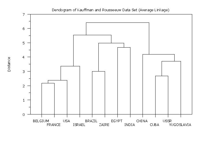
. Step 3:   Generate dendogram from dpst3f.dat file
.
skip 0
read dpst1f.dat indx
read dpst3f.dat xd yd tag
.
orientation portrait
case asis
label case asis
title case asis
title offset 2
label size 1.5
tic mark label size 1.5
title size 1.5
tic mark offset units data
.
let ntemp = size indx
loop for k = 1 1 ntemp
    let itemp = indx(k)
    let string t^k = ^s^itemp
end of loop
let ig = group label t1 to t^ntemp
.
x1label Distance
ylimits 1 12
major ytic mark number 12
minor ytic mark number 0
y1tic mark label format group label
y1tic mark label content ig
ytic mark offset 0.9 0.9
frame corner coordinates 15 20 95 90
.
pre-sort off
horizontal switch on
title Dendogram of Kauffman and Rousseeuw Data Set (Average Linkage)
plot yd xd tag
    



.
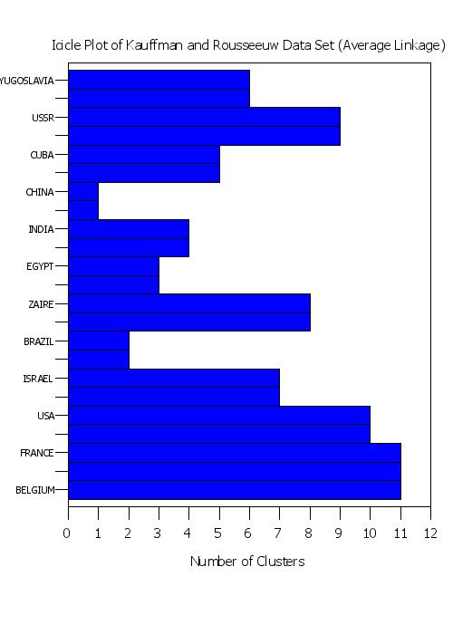
. Step 4:   Generate icicle plot from dpst2f.dat file
.
delete xd yd tag
skip 0
read dpst1f.dat indx
read dpst2f.dat xd yd tag
.
set string space ignore
let ntemp = size indx
let ntic = 2*ntemp - 1
let string tcr = sp()cr()
loop for k = 1 1 ntemp
    let itemp = indx(k)
    let ktemp1 = (k-1)*2 + 1
    let ktemp2 = ktemp1 + 1
    let string t^ktemp1 = ^s^itemp
    if k < ntemp
       let string t^ktemp2 = sp()
    end of if
end of loop
let ig = group label t1 to t^ntic
.
ylimits 1 ntic
major ytic mark number ntic
minor ytic mark number 0
y1tic mark label format group label
y1tic mark label content ig
ytic mark offset 0.9 0.9
frame corner coordinates 15 20 95 90
.
xlimits 0 12
major x1tic mark number 13
minor x1tic mark number 0
.
line blank all
character blank all
bar on all
bar fill on all
bar fill color blue all
.
x1label Number of Clusters
title Icicle Plot of Kauffman and Rousseeuw Data Set (Average Linkage)
plot yd xd tag
    

case asis
label case asis
title case asis
title offset 2
.
. Step 1:   Read the data - a dissimilarity matrix
.
dimension 100 columns
set write decimals 3
.
skip 25
read matrix rouss1.dat y
skip 0
.
let string s1  = Belgium
let string s2  = Brazil
let string s3  = China
let string s4  = Cuba
let string s5  = Egypt
let string s6  = France
let string s7  = India
let string s8  = Israel
let string s9  = USA
let string s10 = USSR
let string s11 = Yugoslavia
let string s12 = Zaire
.
. Step 2:   Perform the agnes cluster analysis
.
set agnes cluster banner plot on
set agnes cluster method average linkage
agnes y
    

The following output is generated

           **********************************************
           *                                            *
           *  ROUSSEEUW/KAUFFMAN AGGLOMERATIVE NESTING  *
           *  CLUSTERING (USING THE AGNES ROUTINE).     *
           *                                            *
           *  DATA IS A DISSIMILARITY MATRIX.           *
           *                                            *
           *  USE AVERAGE LINKAGE METHOD.               *
           *                                            *
           **********************************************
  
  
  
 DISSIMILARITY MATRIX
 -------------------------
  
 001
 002       5.58
 003       7.00     6.50
 004       7.08     7.00     3.83
 005       4.83     5.08     8.17     5.83
 006       2.17     5.75     6.67     6.92     4.92
 007       6.42     5.00     5.58     6.00     4.67     6.42
 008       3.42     5.50     6.42     6.42     5.00     3.92     6.17
 009       2.50     4.92     6.25     7.33     4.50     2.25     6.33     2.75
 010       6.08     6.67     4.25     2.67     6.00     6.17     6.17     6.92
           6.17
 011       5.25     6.83     4.50     3.75     5.75     5.42     6.08     5.83
           6.67     3.67
 012       4.75     3.00     6.08     6.67     5.00     5.58     4.83     6.17
           5.67     6.50     6.92
  
  
  
  
  
 CLUSTER RESULTS
 ---------------
  
  
 THE FINAL ORDERING OF THE OBJECTS IS
  
         1              6              9              8              2
        12              5              7              3              4
        10             11
  
  
 THE DISSIMILARITIES BETWEEN CLUSTERS ARE
  
              2.170          2.375          3.363          5.532          3.000
              4.978          4.670          6.417          4.193          2.670
              3.710
  
  
  
                                   ************
                                   *          *
                                   *  BANNER  *
                                   *          *
                                   ************
  
  
 0  0  0  0  0  0  0  0  0  0  0  0  0  0  0  0  0  0  0  0  0  0  0  0  0  1
 .  .  .  .  .  .  .  .  .  .  .  .  .  .  .  .  .  .  .  .  .  .  .  .  .  .
 0  0  0  1  1  2  2  2  3  3  4  4  4  5  5  6  6  6  7  7  8  8  8  9  9  0
 0  4  8  2  6  0  4  8  2  6  0  4  8  2  6  0  4  8  2  6  0  4  8  2  6  0
  
  
                           001+001+001+001+001+001+001+001+001+001+001+001+001+0
                           *****************************************************
                           006+006+006+006+006+006+006+006+006+006+006+006+006+0
                             ***************************************************
                             009+009+009+009+009+009+009+009+009+009+009+009+009
                                         ***************************************
                                         008+008+008+008+008+008+008+008+008+008
                                                                  **************
                                     002+002+002+002+002+002+002+002+002+002+002
                                     *******************************************
                                     012+012+012+012+012+012+012+012+012+012+012
                                                            ********************
                                                        005+005+005+005+005+005+
                                                        ************************
                                                        007+007+007+007+007+007+
                                                                             ***
                                                   003+003+003+003+003+003+003+0
                                                   *****************************
                                 004+004+004+004+004+004+004+004+004+004+004+004
                                 ***********************************************
                                 010+010+010+010+010+010+010+010+010+010+010+010
                                             ***********************************
                                             011+011+011+011+011+011+011+011+011
 0  0  0  0  0  0  0  0  0  0  0  0  0  0  0  0  0  0  0  0  0  0  0  0  0  1
 .  .  .  .  .  .  .  .  .  .  .  .  .  .  .  .  .  .  .  .  .  .  .  .  .  .
 0  0  0  1  1  2  2  2  3  3  4  4  4  5  5  6  6  6  7  7  8  8  8  9  9  0
 0  4  8  2  6  0  4  8  2  6  0  4  8  2  6  0  4  8  2  6  0  4  8  2  6  0
  
  
  THE ACTUAL HIGHEST LEVEL IS                6.4171875000
  
  
  THE AGGLOMERATIVE COEFFICIENT OF THIS DATA SET IS   0.50
    

.
. Step 3:   Generate dendogram from dpst3f.dat file
.
skip 0
read dpst1f.dat indx
read dpst3f.dat xd yd tag
.
let ntemp = size indx
let string tcr = sp()cr()
loop for k = 1 1 ntemp
    let itemp = indx(k)
    let string t^k = ^s^itemp
    let ival1 = mod(k,2)
    if ival1 = 0
       let t^k = string concatenate tcr t^k
    end of if
end of loop
let ig = group label t1 to t^ntemp
.
xlimits 1 12
major xtic mark number 12
minor xtic mark number 0
x1tic mark label format group label
x1tic mark label content ig
xtic mark offset 0.9 0.9
frame corner coordinates 15 20 95 90
.
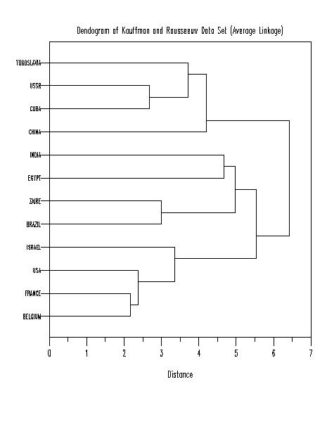
y1label Distance
title Dendogram of Kauffman and Rousseeuw Data Set (Average Linkage)
plot yd xd tag
    



.
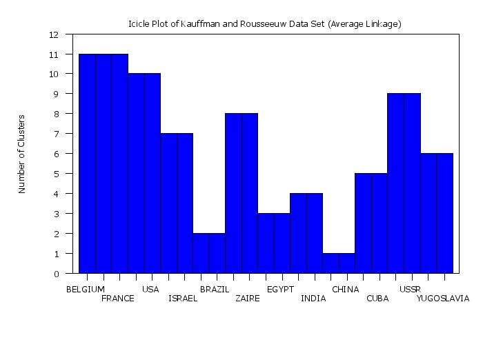
. Step 4:   Generate icicle plot from dpst2f.dat file
.
delete xd yd tag
skip 0
read dpst1f.dat indx
read dpst2f.dat xd yd tag
.
set string space ignore
let ntemp = size indx
let ntic = 2*ntemp - 1
let string tcr = sp()cr()
loop for k = 1 1 ntemp
    let itemp = indx(k)
    let ktemp1 = (k-1)*2 + 1
    let ktemp2 = ktemp1 + 1
    let string t^ktemp1 = ^s^itemp
    if k < ntemp
       let string t^ktemp2 = sp()
    end of if
    let ival1 = mod(k,2)
    if ival1 = 0
       let t^ktemp1 = string concatenate tcr t^ktemp1
    end of if
end of loop
let ig = group label t1 to t^ntic
.
xlimits 1 ntic
major xtic mark number ntic
minor xtic mark number 0
x1tic mark label format group label
x1tic mark label content ig
xtic mark offset 0.9 0.9
frame corner coordinates 15 20 95 90
.
ylimits 0 12
major y1tic mark number 13
minor y1tic mark number 0
.
line blank all
character blank all
bar on all
bar fill on all
bar fill color blue all
.
y1label Number of Clusters
title Icicle Plot of Kauffman and Rousseeuw Data Set (Average Linkage)
plot yd xd tag