1. Exploratory Data Analysis
1.4. EDA Case Studies
1.4.2. Case Studies
1.4.2.5. Beam Deflections

1.4.2.5.4.

Validate New Model

4-Plot of Residuals

The first step in evaluating the fit is to generate a 4-plot of the residuals.

Interpretation

The assumptions are addressed by the graphics shown above:

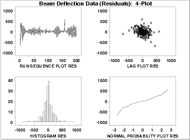
1. The run sequence plot (upper left) indicates that the data do not have any significant shifts in location. There does seem to be some shifts in scale. A start-up effect was detected previously by the complex demodulation amplitude plot. There does appear to be a few outliers.

2. The lag plot (upper right) shows that the data are random. The outliers also appear in the lag plot.

3. The histogram (lower left) and the normal probability plot (lower right) do not show any serious non-normality in the residuals. However, the bend in the left portion of the normal probability plot shows some cause for concern.

The 4-plot indicates that this fit is reasonably good. However, we will attempt to improve the fit by removing the outliers.

Fit Results with Outliers Removed

The following parameter estimates were obtained after removing three outliers.

      Coefficient     Estimate     Stan. Error     t-Value
         C            -178.788        10.57         -16.91
         AMP          -361.759        25.45         -14.22
         FREQ         0.302597      0.1457E-03     2077.00
         PHASE         1.46533      0.4715E-01       31.08
 
      Residual Standard Deviation = 148.3398
      Residual Degrees of Freedom = 193  

New Fit to Edited Data

The original fit, with a residual standard deviation of 155.84, was:

\( \hat{Y}_i = -178.786 - 361.766[2\pi(0.302596)T_i + 1.46536] \)

The new fit, with a residual standard deviation of 148.34, is:

\( \hat{Y}_i = -178.788 - 361.759[2\pi(0.302597)T_i + 1.46533] \)

There is minimal change in the parameter estimates and about a 5 % reduction in the residual standard deviation. In this case, removing the residuals has a modest benefit in terms of reducing the variability of the model.

4-Plot for New Fit

This plot shows that the underlying assumptions are satisfied and therefore the new fit is a good descriptor of the data.

In this case, it is a judgment call whether to use the fit with or without the outliers removed.