1. Exploratory Data Analysis
1.4. EDA Case Studies
1.4.2. Case Studies
1.4.2.2. Uniform Random Numbers

1.4.2.2.2.

Graphical Output and Interpretation

Goal

The goal of this analysis is threefold:

1. Determine if the univariate model:
   \( Y_{i} = C + E_{i} \)

   is appropriate and valid.

2. Determine if the typical underlying assumptions for an "in control" measurement process are valid. These assumptions are:
   1. random drawings;
   2. from a fixed distribution;
   3. with the distribution having a fixed location; and
   4. the distribution having a fixed scale.
3. Determine if the confidence interval
   \( \bar{Y} \pm 2s/\sqrt{N} \)

   is appropriate and valid where s is the standard deviation of the original data.

4-Plot of Data

Interpretation

The assumptions are addressed by the graphics shown above:

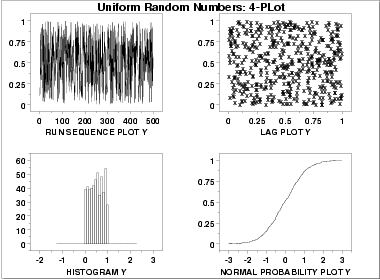
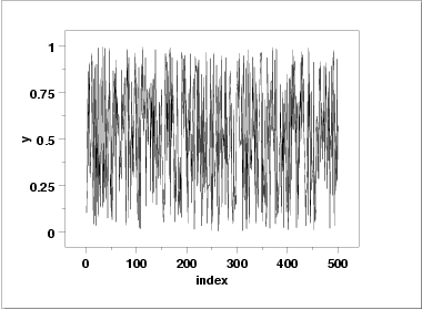
1. The run sequence plot (upper left) indicates that the data do not have any significant shifts in location or scale over time.

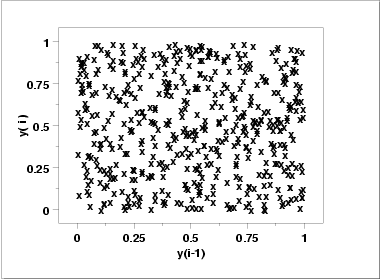
2. The lag plot (upper right) does not indicate any non-random pattern in the data.

3. The histogram shows that the frequencies are relatively flat across the range of the data. This suggests that the uniform distribution might provide a better distributional fit than the normal distribution.

4. The normal probability plot verifies that an assumption of normality is not reasonable. In this case, the 4-plot should be followed up by a uniform probability plot to determine if it provides a better fit to the data. This is shown below.

From the above plots, we conclude that the underlying assumptions are valid. Therefore, the model Y_i = C + E_i is valid. However, since the data are not normally distributed, using the mean as an estimate of C and the confidence interval cited above for quantifying its uncertainty are not valid or appropriate.

Individual Plots

Although it is usually not necessary, the plots can be generated individually to give more detail.

Run Sequence Plot

Lag Plot

Histogram (with overlaid Normal PDF)

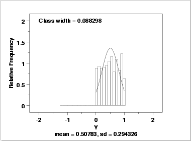
This plot shows that a normal distribution is a poor fit. The flatness of the histogram suggests that a uniform distribution might be a better fit.

Histogram (with overlaid Uniform PDF)

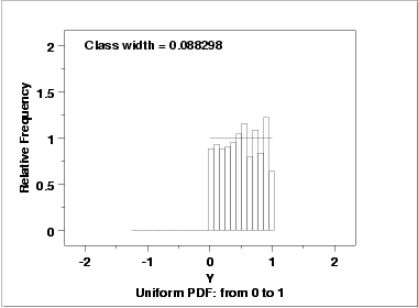
Since the histogram from the 4-plot suggested that the uniform distribution might be a good fit, we overlay a uniform distribution on top of the histogram. This indicates a much better fit than a normal distribution.

Normal Probability Plot

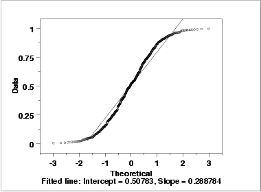
As with the histogram, the normal probability plot shows that the normal distribution does not fit these data well.

Uniform Probability Plot

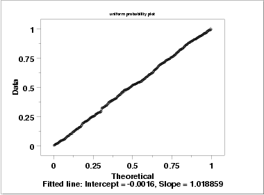
Since the above plots suggested that a uniform distribution might be appropriate, we generate a uniform probability plot. This plot shows that the uniform distribution provides an excellent fit to the data.

Better Model

Since the data follow the underlying assumptions, but with a uniform distribution rather than a normal distribution, we would still like to characterize C by a typical value plus or minus a confidence interval. In this case, we would like to find a location estimator with the smallest variability.

The bootstrap plot is an ideal tool for this purpose. The following plots show the bootstrap plot, with the corresponding histogram, for the mean, median, mid-range, and median absolute deviation.

Bootstrap Plots

Mid-Range is Best

From the above histograms, it is obvious that for these data, the mid-range is far superior to the mean or median as an estimate for location.

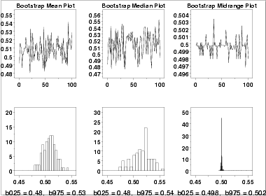
Using the mean, the location estimate is 0.507 and a 95% confidence interval for the mean is (0.482,0.534). Using the mid-range, the location estimate is 0.499 and the 95% confidence interval for the mid-range is (0.497,0.503).

Although the values for the location are similar, the difference in the uncertainty intervals is quite large.

Note that in the case of a uniform distribution it is known theoretically that the mid-range is the best linear unbiased estimator for location. However, in many applications, the most appropriate estimator will not be known or it will be mathematically intractable to determine a valid condfidence interval. The bootstrap provides a method for determining (and comparing) confidence intervals in these cases.