ZIPPPF

ZIPPPF (LET)

Library Function

Compute the Zipf percent point function.

The Zipf distribution has the following probability mass function:

with and n denoting the shape parameters.

Some sources parameterize this distribution with s = - 1 (so that the distribution is defined for s > 0).

The cumulative distribution is computed by summing the probability mass function. The percent point function is the inverse of the cumulative distribution function and is obtained by computing the cumulative distribution until the specified probability is obtained.

LET <y> = ZIPPPF(<p>,<alpha>,<n>)
                        <SUBSET/EXCEPT/FOR qualification>
where <p> is a variable, number, or parameter in the range (0,1);
            <alpha> is a number or parameter greater than 1 that specifies the first shape parameter;
            <n> is a number or parameter that is a positive integer that specifies the second shape parameter;
            <y> is a variable or a parameter where the computed Zipf ppf value is stored;
and where the <SUBSET/EXCEPT/FOR qualification> is optional.

LET A = ZIPPPF(0.95,1.5,100)
LET Y = ZIPPPF(X1,2.3,1000)
PLOT ZIPPPF(X,2.3,100) FOR X = 1 1 100

None

None

ZIPCDF	= Compute the Zipf cumulative distribution function.
ZIPPDF	= Compute the Zipf probability mass function.
ZETPDF	= Compute the Zeta probability mass function.
YULPDF	= Compute the Yule probability mass function.
BGEPDF	= Compute the beta-geometric (Waring) probability mass function.
BTAPDF	= Compute the Borel-Tanner probability mass function.
DLGPDF	= Compute the logarithmic series probability mass function.

Johnson, Kotz, and Kemp (1992), "Univariate Discrete Distributions", Second Edition, Wiley, pp. 465-471.

Distributional Modeling

2006/5

 
multiplot corner coordinates 0 0 100 95
multiplot scale factor 2
case asis
label case asis
title case asis
tic offset units screen
tic offset 3 3
title displacement 2
y1label displacement 17
x1label displacement 12
.
x1label Probability
xlimits 0 1
major xtic mark number 6
minor xtic mark number 3
y1label X
line blank
spike on
.
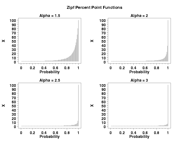
multiplot 2 2
let n = 100
.
let alpha = 1.5
title Alpha = ^alpha
plot zipppf(p,alpha,n) for p = 0  0.01  1
.
let alpha = 2.0
title Alpha = ^alpha
plot zipppf(p,alpha,n) for p = 0  0.01  1
.
let alpha = 2.5
title Alpha = ^alpha
plot zipppf(p,alpha,n) for p = 0  0.01  1
.
let alpha = 3.0
title Alpha = ^alpha
plot zipppf(p,alpha,n) for p = 0  0.01  1
.
end of multiplot
.
justification center
move 50 97
text Zipf Percent Point Functions