ZIPPDF
Name:
Type:
Purpose:
Compute the Zipf probability mass function.
Description:
The Zipf distribution has the following probability mass
function:
with  and n denoting the shape parameters.
Some sources parameterize this distribution with
s =
 - 1
(so that the distribution is defined for s > 0). - 1
(so that the distribution is defined for s > 0).
The mean of the Zipf distribution is
The development of the Zipf distribution was motivated by
Zipf's law (from the linguistics community). Zipf's law
states that the frequency of occurence of any word is
approximately inversely proportional to its rank in the
frequency table. When Zipf's law is applicable, plotting
the frequency table on a log-log scale (i.e., log(frequency)
versus log(rank order)) will typically show a linear pattern.
Note that Zipf's law is an empirical (as oppossed to a
theoretical) law. However, Zipf's law has served as a
useful model for many different kinds of phenomena.
Syntax:
LET <y> = ZIPPDF(<x>,<alpha>,<n>)
<SUBSET/EXCEPT/FOR qualification>
where <x> is a positive integer variable, number, or
parameter;
<alpha> is a number or parameter greater than 1 that
specifies the first shape parameter;
<n> is a number or parameter that is a positive integer
that specifies the second shape parameter;
<y> is a variable or a parameter where the computed
Zipf pdf value is stored;
and where the <SUBSET/EXCEPT/FOR qualification> is optional.
Examples:
LET A = ZIPPDF(3,1.5,100)
LET Y = ZIPPDF(X1,2.3,1000)
PLOT ZIPPDF(X,2.3,100) FOR X = 1 1 100
Note:
The zeta distribution is the
limiting case of the Zipf distribution as n goes to
infinity. Note that zeta distribution and Zipf distribution
tend to be used interchangeably in the literature. The primary
distinction is that the Zipf distribution is bounded in the
upper tail while the zeta distribution is unbounded in the upper
tail. When the upper bound for the Zipf distribution is large,
the zeta distribution is typically used as an approximation.
Note:
For a number of commands utilizing the zeta distribution,
it is convenient to bin the data. There are two basic ways
of binning the data.
- For some commands (histograms, maximum likelihood
estimation), bins with equal size widths are required.
This can be accomplished with the following commands:
LET AMIN = MINIMUM Y
LET AMAX = MAXIMUM Y
LET AMIN2 = AMIN - 0.5
LET AMAX2 = AMAX + 0.5
CLASS MINIMUM AMIN2
CLASS MAXIMUM AMAX2
CLASS WIDTH 1
LET Y2 X2 = BINNED Y
- For some commands, unequal width bins may be
helpful. In particular, for the chi-square goodness
of fit, it is typically recommended that the minimum
class frequency be at least 5. In this case, it may
be helpful to combine small frequencies in the tails.
Unequal class width bins can be created with the
commands
LET MINSIZE = <value>
LET Y3 XLOW XHIGH = INTEGER FREQUENCY TABLE Y
If you already have equal width bins data, you can
use the commands
LET MINSIZE = <value>
LET Y3 XLOW XHIGH = COMBINE FREQUENCY TABLE Y2 X2
The MINSIZE parameter defines the minimum class
frequency. The default value is 5.
Note:
You can generate Zipf random numbers and probability
plots with the following commands:
LET NLAST = <value>
LET N = <value>
LET ALPHA = <value>
LET Y = ZIPF RANDOM NUMBERS FOR I = 1 1 NLAST
ZIPF PROBABILITY PLOT Y
ZIPF PROBABILITY PLOT Y2 X2
ZIPF PROBABILITY PLOT Y3 XLOW XHIGH
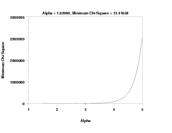
You can generate an estimate of alpha, assuming the value
of n is known, based on the maximum ppcc value or the
minimum chi-square goodness of fit with the commands
LET N = <value>
LET ALPHA1 = <value>
LET ALPHA2 = <value>
ZIPF KS PLOT Y
ZIPF KS PLOT Y2 X2
ZIPF KS PLOT Y3 XLOW XHIGH
ZIPF PPCC PLOT Y
ZIPF PPCC PLOT Y2 X2
ZIPF PPCC PLOT Y3 XLOW XHIGH
If the value of n is unknown, you can use the maximum
data value as the estimate of n. The default values of
ALPHA1 and ALPHA2 are 1.5 and 5, respectively. Due to the
discrete nature of the percent point function for discrete
distributions, the ppcc plot will not be smooth. For that
reason, if there is sufficient sample size the KS PLOT (i.e.,
the minimum chi-square value) is typically preferred. Also,
since the data is integer values, one of the binned forms is
preferred for these commands.
To generate a chi-square goodness of fit test, enter the
commands
LET N = <value>
LET ALPHA = <value>
ZIPF CHI-SQUARE GOODNESS OF FIT Y2 X2
ZIPF CHI-SQUARE GOODNESS OF FIT Y3 XLOW XHIGH
Default:
Synonyms:
Related Commands:
|
ZIPCDF
|
= Compute the Zipf cumulative distribution function.
|
|
ZIPPPF
|
= Compute the Zipf percent point function.
|
|
ZETPDF
|
= Compute the Zeta probability mass function.
|
|
YULPDF
|
= Compute the Yule probability mass function.
|
|
BGEPDF
|
= Compute the beta-geometric (Waring) probability mass
function.
|
|
BTAPDF
|
= Compute the Borel-Tanner probability mass function.
|
|
DLGPDF
|
= Compute the logarithmic series probability mass function.
|
|
INTEGER FREQUENCY TABLE
|
= Generate a frequency table at
|
|
COMBINE FREQUENCY TABLE
|
= Combine low frequency classes in a frequency table.
|
|
KS PLOT
|
= Generate a minimum chi-square plot.
|
|
MAXIMUM
LIKELIHOOD
|
= Perform maximum likelihood estimation for a
distribution.
|
Reference:
Johnson, Kotz, and Kemp (1992), "Univariate Discrete
Distributions", Second Edition, Wiley, pp. 465-471.
Applications:
Implementation Date:
Program:
let n = 100
let alpha = 1.7
let y = zipf random numbers for i = 1 1 500
.
let y3 xlow xhigh = integer frequency table y
class lower 0.5
class width 1
let amax = maximum y
let amax2 = amax + 0.5
class upper amax2
let y2 x2 = binned y
.
label case asis
x1label Alpha
y1label Minimum Chi-Square
zipf ks plot y3 xlow xhigh
let alpha = shape
case asis
justification center
move 50 92
text Alpha = ^alpha, Minimum Chi-Square = ^minks
zipf chi-square goodness of fit y3 xlow xhigh
.
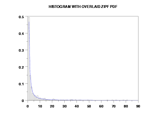
title Histogram with Overlaid Zipf PDF
label
relative histogram y2 x2
limits freeze
pre-erase off
line color blue
plot zippdf(x,alpha,n) for x = 1 1 n
limits
pre-erase on
line color black


                   CHI-SQUARED GOODNESS-OF-FIT TEST

 NULL HYPOTHESIS H0:      DISTRIBUTION FITS THE DATA
 ALTERNATE HYPOTHESIS HA: DISTRIBUTION DOES NOT FIT THE DATA
 DISTRIBUTION:            ZIPF

 SAMPLE:
    NUMBER OF OBSERVATIONS      =      500
    NUMBER OF NON-EMPTY CELLS   =       18
    NUMBER OF PARAMETERS USED   =        1

 TEST:
 CHI-SQUARED TEST STATISTIC     =    13.41658
    DEGREES OF FREEDOM          =       16
    CHI-SQUARED CDF VALUE       =    0.357910

    ALPHA LEVEL         CUTOFF              CONCLUSION
            10%       23.54183               ACCEPT H0
             5%       26.29623               ACCEPT H0
             1%       31.99993               ACCEPT H0

       CELL NUMBER, LOWER BIN POINT, UPPER BIN POINT, OBSERVED FREQUENCY, AND EXPECTED FREQUENCY
       WRITTEN TO FILE DPST1F.DAT
Date created: 6/5/2006
Last updated: 6/5/2006
Please email comments on this WWW page to
[email protected].
|


![p(x;alpha,n) = (1/x^alpha)/SUM[i=1 to n][1/i**alpha]
x = 1, 2, ..., n; alpha > 1; n a positive integer](eqns/zippdf.gif)
![mean = SUM[i=1 to n][1/i**(alpha-2)]/SUM[i=1 to n][1/i**(alpha-1)]
alpha > 2](eqns/zipfmean.gif)
