SED navigation bar go to SED home page go to Dataplot home page go to NIST home page SED Home Page SED Staff SED Projects SED Products and Publications Search SED Pages
Dataplot Vol 2 Vol 1

RELATIVE RISK

Name:
    RELATIVE RISK (LET)
Type:
    Let Subcommand
Purpose:
    Compute the relative risk between two binary variables.
Description:
    Given two variables with n parired observations where each variable has exactly two possible outcomes, we can generate the following 2x2 table:

        Variable 2  
      Variable 1 Success Failure Row Total

      Success N11 N12 N11 + N12
      Failure N21 N22 N21 + N22

      Column Total N11 + N21 N12 + N22 N

    The parameters N11, N12, N21, and N22 denote the counts for each category.

    Success and failure can denote any binary response. Dataplot expects "success" to be coded as "1" and "failure" to be coded as "0". Some typical examples would be:

    1. Variable 1 denotes whether or not a patient has a disease (1 denotes disease is present, 0 denotes disease not present). Variable 2 denotes the result of a test to detect the disease (1 denotes a positive result and 0 denotes a negative result).

    2. Variable 1 denotes whether an object is present or not (1 denotes present, 0 denotes absent). Variable 2 denotes a detection device (1 denotes object detected and 0 denotes object not detected).

    In these examples, the "ground truth" is typically given as variable 1 while some estimator of the ground truth is given as variable 2.

    The relative risk is defined as the ratio of the probability of "success" probabilities, that is

      relative risk = {N11/(N11 + N21)}/{N12/(N12 + N22)}

    The relative risk is a useful statistic when comparing the difference in two binomial proportions when the probabilities of success are close to zero. For example, page 21 of Agresti gives the example where the absolute difference of proportions between 0.410, 0.401 and 0.010, 0.001 are both 0.09. However the relative risks are 0.410/0.401 = 1.02 and 0.010/0.001 = 10.

Syntax:
    LET <par> = RELATIVE RISK <y1> <y2>
                            <SUBSET/EXCEPT/FOR qualification>
    where <y1> is the first response variable;
                <y2> is the second response variable;
                <par> is a parameter where the computed relative risk is stored;
    and where the <SUBSET/EXCEPT/FOR qualification> is optional.
Examples:
    LET A = RELATIVE RISK Y1 Y2
    LET A = RELATIVE RISK Y1 Y2 SUBSET TAG > 2
Note:
    The two variables need not have the same number of elements.
Note:
    There are two ways you can define the response variables:

    1. Raw data - in this case, the variables contain 0's and 1's.

      If the data is not coded as 0's and 1's, Dataplot will check for the number of distinct values. If there are two distinct values, the minimum value is converted to 0's and the maximum value is converted to 1's. If there is a single distinct value, it is converted to 0's if it is less than 0.5 and to 1's if it is greater than or equal to 0.5. If there are more than two distinct values, an error is returned.

    2. Summary data - if there are two observations, the data is assummed to be the 2x2 summary table. That is,

        Y1(1) = N11
        Y1(2) = N21
        Y2(1) = N12
        Y2(2) = N22

    Note that the above commands expect the variables to have the same number of observations. If the two samples are in fact of different sizes, there are two ways to address the issue:

    1. Y1 and Y2 can contain the summary data. That is,

        Y1(1) = N11
        Y1(2) = N21
        Y2(1) = N12
        Y2(2) = N22

      This is a useful option in that the data is sometimes only available in summary form. Note that this will not work for the BOOTSTRAP PLOT and JACKNIFE PLOT commands (these require raw data).

    2. You can specify a missing value for the smaller sample. For example, if Y1 has 100 observations and Y2 has 200 observations, you can do something like

        SET STATISTIC MISSING VALUE -99
        LET Y1 = -99 FOR I = 101 1 200
Note:
    Dataplot statistics can be used in 20+ commands. For details, enter

Default:
    None
Synonyms:
    None
Related Commands: Reference:
    Fleiss, Levin, and Paik (2003), "Statistical Methods for Rates and Proportions", Third Edition, Wiley, chapter 1.

    Agresti (2007), "Introduction to Categorical Data Analysis", Second Edition, Wiley.

Applications:
    Categorical Data Analysis
Implementation Date:
    2007/04
Program:
     
    let n = 1
    .
    let p = 0.2
    let y1 = binomial rand numb for i = 1 1 100
    let p = 0.1
    let y2 = binomial rand numb for i = 1 1 100
    .
    let p = 0.4
    let y1 = binomial rand numb for i = 101 1 200
    let p = 0.08
    let y2 = binomial rand numb for i = 101 1 200
    .
    let p = 0.15
    let y1 = binomial rand numb for i = 201 1 300
    let p = 0.18
    let y2 = binomial rand numb for i = 201 1 300
    .
    let p = 0.6
    let y1 = binomial rand numb for i = 301 1 400
    let p = 0.45
    let y2 = binomial rand numb for i = 301 1 400
    .
    let p = 0.3
    let y1 = binomial rand numb for i = 401 1 500
    let p = 0.1
    let y2 = binomial rand numb for i = 401 1 500
    .
    let x = sequence 1 100 1 5
    .
    let a = relative risk y1 y2 subset x = 1
    tabulate relative risk y1 y2 x
    .
    label case asis
    xlimits 1 5
    major xtic mark number 5
    minor xtic mark number 0
    xtic mark offset 0.5 0.5
    y1label Relative Risk
    x1label Group ID
    character x blank
    line blank solid
    .
    relative risk plot y1 y2 x
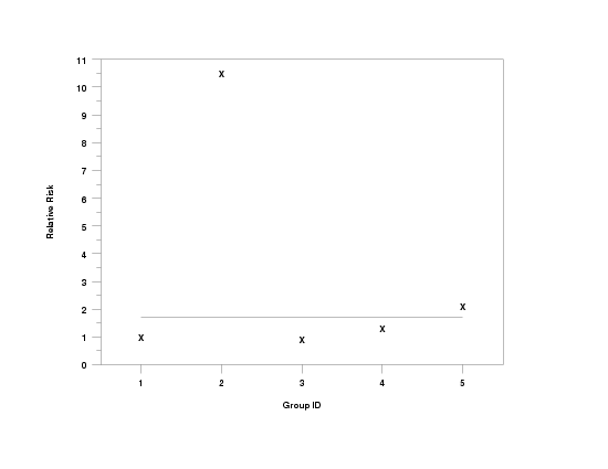
        
    plot generated by sample program

Privacy Policy/Security Notice
Disclaimer | FOIA

NIST is an agency of the U.S. Commerce Department.

Date created: 07/24/2007
Last updated: 10/07/2016

Please email comments on this WWW page to alan.heckert@nist.gov.