GTLPDF

GTLPDF (LET)

Library Function

Compute the generalized Topp and Leone probability density function with shape parameters and .

The generalized Topp and Leone distribution has the following probability density function:

with and denoting the shape parameters and a and b the lower and upper limits, respectively.

The case where a = 0 and b = 1 is referred to as the standard generalized Topp and Leone distribution. It has the following probability density function:

The lower and upper limits are related to the location and scale parameters as follows:

location = a
scale = b - a


Kotz and van Dorp have proposed this distribution as an alternative to the beta distribution.

LET <y> = GTLPDF(<x>,<alpha>,<beta>,<a>,<b>)
                        <SUBSET/EXCEPT/FOR qualification>
where <x> is a number, parameter, or variable containing values in the interval (a,b);
            <y> is a variable or a parameter (depending on what <x> is) where the computed generalized Topp and Leone pdf value is stored;
            <alpha> is a number, parameter, or variable in the interval (0, 2) that specifies the first shape parameter;
            <beta> is a positive number, parameter, or variable that specifies the second shape parameter;
            <a> is a number, parameter, or variable that specifies the lower limit;
            <b> is a number, parameter, or variable that specifies the upper limit;
and where the <SUBSET/EXCEPT/FOR qualification> is optional.

If <a> and <b> are omitted, they default to 0 and 1, respectively.

LET A = GTLPDF(0.3,0.2,1.2)
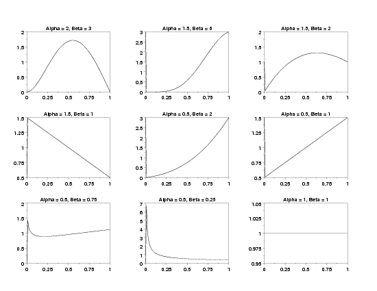
LET Y = GTLPDF(X,0.5,2)
PLOT GTLPDF(X,2,3) FOR X = 0 0.01 1

Generalized Topp and Leone random numbers, probability plots, and goodness of fit tests can be generated with the commands:
LET ALPHA = <value>
LET BETA = <value>
LET A = <value>
LET B = <value>
LET Y = GENERALIZED TOPP LEONE ...
                RANDOM NUMBERS FOR I = 1 1 N
GENERALIZED TOPP LEONE PROBABILITY PLOT Y
GENERALIZED TOPP LEONE PROBABILITY PLOT Y2 X2
GENERALIZED TOPP LEONE PROBABILITY PLOT Y3 XLOW XHIGH
GENERALIZED TOPP LEONE ...
                KOLMOGOROV SMIRNOV GOODNESS OF FIT Y
GENERALIZED TOPP LEONE CHI-SQUARE GOODNESS OF FIT Y2 X2
GENERALIZED TOPP LEONE CHI-SQUARE ...
                GOODNESS OF FIT Y3 XLOW XHIGH


The following commands can be used to estimate the and shape parameters for the generalized Topp and Leone distribution:

LET ALPHA1 = <value>$
LET ALPHA2 = <value>$
LET BETA1 = <value>$
LET BETA2 = <value>$
GENERALIZED TOPP LEONE PPCC PLOT Y$
GENERALIZED TOPP LEONE PPCC PLOT Y2 X2$
GENERALIZED TOPP LEONE PPCC PLOT Y3 XLOW XHIGH$
GENERALIZED TOPP LEONE KS PLOT Y$
GENERALIZED TOPP LEONE KS PLOT Y2 X2$
GENERALIZED TOPP LEONE KS PLOT Y3 XLOW XHIGH$


The default values for ALPHA1 and ALPHA2 are 0.1 and 2. The default values for BETA1 and BETA2 are 0.5 and 10.

The probability plot can then be used to estimate the lower and upper limits (lower limit = PPA0, upper limit = PPA0 + PPA1).

The following options may be useful for these commands.

1. Instead of generating the ppcc plot or ks plot on the original data, we can generate them on selected percentiles of the data. For example, if we have 1,000 points, we can choose to generate the plots on 100 evenly spaced percentiles with the command
   SET PPCC PLOT DATA POINTS 100

   This can be used to speed up the generation of the plot for larger data sets.

2. For the ks plot, we can fix the location and scale. This is equivalent to assuming that the lower and upper limits are known (e.g., we could use the data minimum and maximum as the lower and upper limit values). Given that the lower and upper limits are LOWLIM and UPPLIM, enter the commands
   LET KSLOC = LOWLIM
   LET KSSCALE = UPPLIM
   

   The ppcc plot is invariant to location and scale, so we cannot fix the lower and upper limits.

None

None

GTLCDF	= Compute the generalized Topp and Leone cumulative distribution function.
GTLPPF	= Compute the generalized Topp and Leone percent point function.
RGTPDF	= Compute the reflected generalized Topp and Leone probability density function.
TOPPDF	= Compute the Topp and Leone probability density function.
TSPPDF	= Compute the two-sided power probability density function.
BETPDF	= Compute the beta probability density function.
TRIPDF	= Compute the triangular probability density function.
TRAPDF	= Compute the trapezoid probability density function.
UNIPDF	= Compute the uniform probability density function.
POWPDF	= Compute the power probability density function.
JSBPDF	JSBPDF = Compute the Johnson SB probability density function.

Samuel Kotz and J. Rene Van Dorp 2004, "Beyond Beta: Other Continuous Families of Distributions with Bounded Support and Applications", World Scientific, chapter 7.

Distributional Modeling

2007/2

 
LABEL CASE ASIS
TITLE CASE ASIS
TITLE OFFSET 2
.
MULTIPLOT 3 3
MULTIPLOT CORNER COORDINATES 0 0 100 95
MULTIPLOT SCALE FACTOR 3
.
LET ALPHA = 2
LET BETA  = 3
TITLE Alpha = ^alpha, Beta = ^beta
PLOT GTLPDF(X,ALPHA,BETA) FOR X = 0  0.01  1
.
LET ALPHA = 1.5
LET BETA  = 6
TITLE Alpha = ^alpha, Beta = ^beta
PLOT GTLPDF(X,ALPHA,BETA) FOR X = 0  0.01  1
.
LET ALPHA = 1.5
LET BETA  = 2
TITLE Alpha = ^alpha, Beta = ^beta
PLOT GTLPDF(X,ALPHA,BETA) FOR X = 0  0.01  1
.
LET ALPHA = 1.5
LET BETA  = 1
TITLE Alpha = ^alpha, Beta = ^beta
PLOT GTLPDF(X,ALPHA,BETA) FOR X = 0  0.01  1
.
LET ALPHA = 0.5
LET BETA  = 2
TITLE Alpha = ^alpha, Beta = ^beta
PLOT GTLPDF(X,ALPHA,BETA) FOR X = 0  0.01  1
.
LET ALPHA = 0.5
LET BETA  = 1
TITLE Alpha = ^alpha, Beta = ^beta
PLOT GTLPDF(X,ALPHA,BETA) FOR X = 0  0.01  1
.
LET ALPHA = 0.5
LET BETA  = 0.75
TITLE Alpha = ^alpha, Beta = ^beta
PLOT GTLPDF(X,ALPHA,BETA) FOR X = 0  0.01  1
.
LET ALPHA = 0.5
LET BETA  = 0.25
TITLE Alpha = ^alpha, Beta = ^beta
PLOT GTLPDF(X,ALPHA,BETA) FOR X = 0  0.01  1
.
LET ALPHA = 1
LET BETA  = 1
TITLE Alpha = ^alpha, Beta = ^beta
PLOT GTLPDF(X,ALPHA,BETA) FOR X = 0  0.01  1
.
END OF MULTIPLOT
    

 
let alpha = 1.5
let beta = 2
.
let y = generalized topp leone rand numb for i = 1 1 200
.
let alphsav = alpha
let betasav = beta
generalized topp leone ppcc plot y
just center
move 50 5
let alpha = shape1
let beta = shape2
text maxppcc = ^maxppcc, Alpha = ^alpha, Beta = ^beta
move 50 2
text Alphasav = ^alphsav, Betasav = ^betasav
.
char x
line blank
generalized topp leone prob plot y
move 50 5
text PPA0 = ^ppa0, PPA1 = ^ppa1
move 50 2
let upplim = ppa0 + ppa1
text Lower Limit = ^ppa0, Upper Limit = ^upplim
char blank
line solid
.
let ksloc = ppa0
let ksscale = upplim
generalized topp leone kolm smir goodness of fit y
.
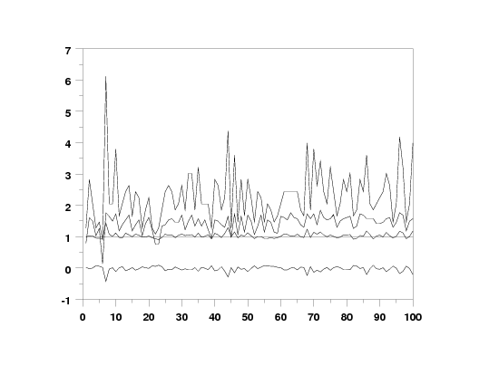
bootstrap generalized topp leone plot y
    

The following output is generated:





                   KOLMOGOROV-SMIRNOV GOODNESS-OF-FIT TEST
  
 NULL HYPOTHESIS H0:      DISTRIBUTION FITS THE DATA
 ALTERNATE HYPOTHESIS HA: DISTRIBUTION DOES NOT FIT THE DATA
 DISTRIBUTION:            GENERALIZED TOPP AND LEONE
    NUMBER OF OBSERVATIONS              =      200
  
 TEST:
 KOLMOGOROV-SMIRNOV TEST STATISTIC      =    1.000000
  
    ALPHA LEVEL         CUTOFF              CONCLUSION
            10%       0.086*              REJECT H0
                      0.085**
             5%       0.096*              REJECT H0
                      0.095**
             1%       0.115*              REJECT H0
                      0.114**
  
     *  - STANDARD LARGE SAMPLE APPROXIMATION  ( C/SQRT(N) )
    ** - MORE ACCURATE LARGE SAMPLE APPROXIMATION  ( C/SQRT(N + SQRT(N/10)) )