SED navigation bar go to SED home page go to Dataplot home page go to NIST home page SED Home Page SED Staff SED Projects SED Products and Publications Search SED Pages
Dataplot Vol 2 Vol 1

DIFFERENCE OF QUANTILE

Name:
    DIFFERENCE OF QUANTILE (LET)
Type:
    Let Subcommand
Purpose:
    Compute the difference between the QUANTILEs for two response variables.
Description:
    The qth quantile of a data set is defined as that value where a q fraction of the data is below that value and (1-q) fraction of the data is above that value. For example, the 0.5 quantile is the median.

    Dataplot supports two methods for computing the quantile.

    The first method is based on the order statistic. The formula is:

      \( \hat{X}_q = (1 - r)X_{NI1} + rX_{NI2} \)

    where

      X are the observations sorted in ascending order
      NI1 = INT(q*(n+1))
      NI2 = NI1 + 1
      r = q*(n+1) - INT(q*(n+1))

    An alternative method is called the Herrell-Davis estimate. This method attempts to provide a lower standard error for Xq by utilizing all the order statistics rather than a single (or a weighted average of two) order statistic. Note that there are caes where the Herrell-Davis has a substantially smaller standard error than the order statistic method. However, there are also cases where the reverse is true.

    To compute the Herrell-Davis estimate, do the following:

    1. Sort the X in ascending order.

    2. A = (n+1)*q

    3. B = (n+1)*(1 - q)

    4. Wi = BETCDF(i/n,A,B) - BETCDF((i-1)/n,A,B) where BETCDF is the beta cumulative distribution function with shape parameters A and B.

    5. \( \hat{X}_q = \sum_{i=1}^{n}{W_{i}X_{i}} \)

    For the difference of quantiles, the quantile is computed for each of two samples then their difference is taken.

Syntax:
    LET <par> = DIFFERENCE OF QUANTILE <y1> <y2>
                            <SUBSET/EXCEPT/FOR qualification>
    where <y1> is the first response variable;
                <y2> is the first response variable;
                <par> is a parameter where the computed difference of the quantiles is stored;
    and where the <SUBSET/EXCEPT/FOR qualification> is optional.
Examples:
    LET A = DIFFERENCE OF QUANTILE Y1 Y2
    LET A = DIFFERENCE OF QUANTILE Y1 Y2 SUBSET X > 1
Note:
    The following command is used to determine which method is used to compute the quantile:

      SET QUANTILE METHOD <ORDER/HERRELL-DAVIS>
Note:
    The specific quantile to compute is specified by entering the following command:

      LET XQ = <value>

    where <value> is a number in the interval (0,1) that specifies the desired quantile.

Note:
    Dataplot statistics can be used in a number of commands. For details, enter

Default:
    None
Synonyms:
    None
Related Commands: Reference:
    Rand Wilcox (1997), "Introduction to Robust Estimation and Hypothesis Testing," Academic Press.

    Frank Herrell and C. E. Davis (1982), "A New Distribution-Free Quantile Estimator," Biometrika, 69(3), 635-640.

Applications:
    Data Analysis
Implementation Date:
    2003/03
Program:
    SKIP 25 
    READ IRIS.DAT Y1 TO Y4 X 
    . 
    LET XQ = 0.9 
    . 
    LET A = DIFFERENCE OF QUANTILE Y1 Y2 
    TABULATE DIFFERENCE OF QUANTILE Y1 Y2 X 
    . 
    XTIC OFFSET 0.2 0.2 
    X1LABEL GROUP ID 
    Y1LABEL DIFFERENCE OF (0.9) QUANTILE 
    CHAR X 
    LINE BLANK 
    DIFFERENCE OF QUANTILE PLOT Y1 Y2 X 
    CHAR X ALL 
    LINE BLANK ALL 
    BOOTSTRAP DIFFERENCE OF QUANTILE PLOT Y1 Y2 X  
        
    Dataplot generated the following output.
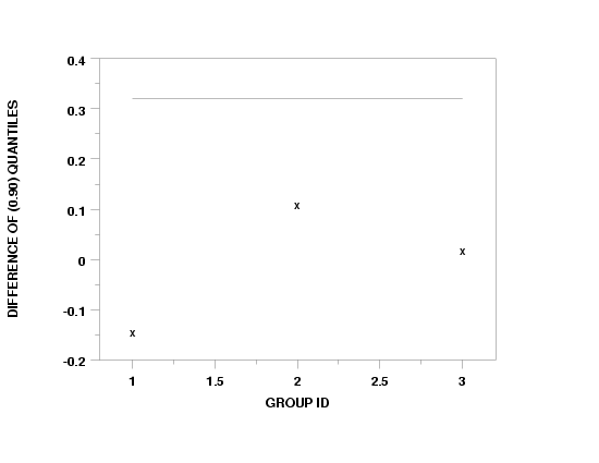
        
    plot generated by sample program

    plot generated by sample program

Privacy Policy/Security Notice
Disclaimer | FOIA

NIST is an agency of the U.S. Commerce Department.

Date created: 03/27/2003
Last updated: 11/12/2015

Please email comments on this WWW page to alan.heckert@nist.gov.