BU6PDF

BU6PDF (LET)

Library Function

Compute the Burr type 6 probability density function with shape parameters r and k.

The standard Burr type 6 distribution has the following probability density function:

with r and k denoting the shape parameters.

This distribution can be generalized with location and scale parameters in the usual way using the relation

LET <y> = BU6PDF(<x>,<r>,<k>,<loc>,<scale>)
                        <SUBSET/EXCEPT/FOR qualification>
where <x> is a number, parameter, or variable;
            <y> is a variable or a parameter (depending on what <x> is) where the computed Burr type 6 pdf value is stored;
            <r> is a positive number, parameter, or variable that specifies the first shape parameter;
            <k> is a positive number, parameter, or variable that specifies the second shape parameter;
            <loc> is a number, parameter, or variable that specifies the location parameter;
            <scale> is a positive number, parameter, or variable that specifies the scale parameter;
and where the <SUBSET/EXCEPT/FOR qualification> is optional.

If <loc> and <scale> are omitted, they default to 0 and 1, respectively.

LET A = BU6PDF(0.3,0.2,1.7)
LET Y = BU6PDF(X,0.5,2.2,0,5)
PLOT BU6PDF(X,2,1.8) FOR X = -5 0.01 5

Burr type 6 random numbers, probability plots, and goodness of fit tests can be generated with the commands:
LET R = <value>
LET K = <value>
LET Y = BURR TYPE 6 RANDOM NUMBERS FOR I = 1 1 N
BURR TYPE 6 PROBABILITY PLOT Y
BURR TYPE 6 PROBABILITY PLOT Y2 X2
BURR TYPE 6 PROBABILITY PLOT Y3 XLOW XHIGH
BURR TYPE 6 KOLMOGOROV SMIRNOV GOODNESS OF FIT Y
BURR TYPE 6 CHI-SQUARE GOODNESS OF FIT Y2 X2
BURR TYPE 6 CHI-SQUARE GOODNESS OF FIT Y3 XLOW XHIGH


The following commands can be used to estimate the r and k shape parameters for the Burr type 6 distribution:

LET R1 = <value>
LET R2 = <value>
LET K1 = <value>
LET K2 = <value>
BURR TYPE 6 PPCC PLOT Y
BURR TYPE 6 PPCC PLOT Y2 X2
BURR TYPE 6 PPCC PLOT Y3 XLOW XHIGH
BURR TYPE 6 KS PLOT Y
BURR TYPE 6 KS PLOT Y2 X2
BURR TYPE 6 KS PLOT Y3 XLOW XHIGH


The default values for R1 and R2 are 0.5 and 10 and the default values for K1 and K2 are 0.5 and 10..

The probability plot can then be used to estimate the location and scale (location = PPA0, scale = PPA1).

The BOOTSTRAP DISTRIBUTION command can be used to find uncertainty intervals for the parameter estimates based on the ppcc plot and ks plot.

None

BURR TYPE VI is a synonym for BURR TYPE 6.

BU6CDF	= Compute the Burr type 6 cumulative distribution function.
BU6PPF	= Compute the Burr type 6 percent point function.
BU2PDF	= Compute the Burr type 2 probability density function.
BU3PDF	= Compute the Burr type 3 probability density function.
BU4PDF	= Compute the Burr type 4 probability density function.
BU5PDF	= Compute the Burr type 5 probability density function.
BU7PDF	= Compute the Burr type 7 probability density function.
BU8PDF	= Compute the Burr type 8 probability density function.
BU9PDF	= Compute the Burr type 9 probability density function.
B10PDF	= Compute the Burr type 10 probability density function.
B11PDF	= Compute the Burr type 11 probability density function.
B12PDF	= Compute the Burr type 12 probability density function.
RAYPDF	= Compute the Rayleigh probability density function.
WEIPDF	= Compute the Weibull probability density function.
EWEPDF	= Compute the exponentiated Weibull probability density function.

Burr (1942), "Cumulative Frequency Functions", Annals of Mathematical Statistics, 13, pp. 215-232.

Johnson, Kotz, and Balakrishnan (1994), "Contiunuous Univariate Distributions--Volume 1", Second Edition, Wiley, pp. 53-54.

Devroye (1986), "Non-Uniform Random Variate Generation", Springer-Verlang, pp. 476-477.

Distributional Modeling

2007/10

 
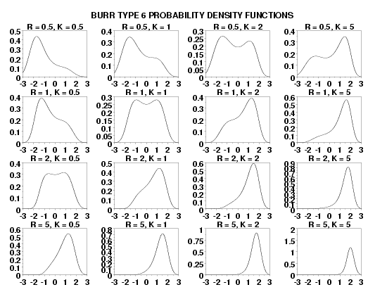
LABEL CASE ASIS
TITLE CASE ASIS
TITLE OFFSET 2
.
MULTIPLOT 4 4
MULTIPLOT CORNER COORDINATES 0 0 100 95
MULTIPLOT SCALE FACTOR 4
.
LET RVAL = DATA 0.5  1  2  5
LET KVAL = DATA 0.5  1  2  5
.
LOOP FOR IROW = 1 1 4
    LOOP FOR ICOL = 1 1 4
        LET R  = RVAL(IROW)
        LET K = KVAL(ICOL)
        TITLE R = ^r, K = ^k
        PLOT BU6PDF(X,R,K) FOR X = -3  0.01  3
    END OF LOOP
END OF LOOP
.
END OF MULTIPLOT
.
JUSTIFICATION CENTER
MOVE 50 97
TEXT Burr Type 6 Probability Density Functions
    

 
let r = 2.1
let k = 1.3
let rsav = r
let ksav = k
.
let y = burr type 6 random numbers for i = 1 1 200
let y = 10*y
let amin = minimum y
let amax = maximum y
.
y1label Correlation Coefficeint
x1label K (Curves Represent Values of R)
let r1 = 0.5
let r2 = 5
let k1 = 0.5
let k2 = 3
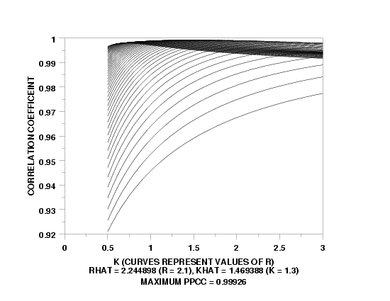
burr type 6 ppcc plot y
let r = shape1
let k = shape2
justification center
move 50 6
text Rhat = ^r (R = ^rsav), Khat = ^k (K = ^ksav)
move 50 2
text Maximum PPCC = ^maxppcc
.
y1label Data
x1label Theoretical
char x
line bl
burr type 6 prob plot y
move 50 6
text Location = ^ppa0, Scale = ^ppa1
char bl
line so
.
let loc = ppa0
let scale = ppa1
.
y1label Relative Frequency
x1label
relative hist y
limits freeze
pre-erase off
line color blue
plot bu6pdf(x,r,k,loc,scale) for x = amin .01 amax
line color black
limits 
pre-erase on
.
let ksloc = loc
let ksscale = scale
burr type 6 kolmogorov smirnov goodness of fit y
    







                   KOLMOGOROV-SMIRNOV GOODNESS-OF-FIT TEST
  
 NULL HYPOTHESIS H0:      DISTRIBUTION FITS THE DATA
 ALTERNATE HYPOTHESIS HA: DISTRIBUTION DOES NOT FIT THE DATA
 DISTRIBUTION:            BURR TYPE 6
    NUMBER OF OBSERVATIONS              =      200
  
 TEST:
 KOLMOGOROV-SMIRNOV TEST STATISTIC      =   0.2968693E-01
  
    ALPHA LEVEL         CUTOFF              CONCLUSION
            10%       0.086*              ACCEPT H0
                      0.085**
             5%       0.096*              ACCEPT H0
                      0.095**
             1%       0.115*              ACCEPT H0
                      0.114**
  
     *  - STANDARD LARGE SAMPLE APPROXIMATION  ( C/SQRT(N) )
    ** - MORE ACCURATE LARGE SAMPLE APPROXIMATION  ( C/SQRT(N + SQRT(N/10)) )