
|
BGECDFName:
 and and
 . .
 and
and  ,
the resulting distribution is referred to as a beta-geometric
distribution. For a standard geometric distribution, p
is assumed to be fixed for successive trials. For the
beta-geometric distribution, the value of p changes
for each trial. ,
the resulting distribution is referred to as a beta-geometric
distribution. For a standard geometric distribution, p
is assumed to be fixed for successive trials. For the
beta-geometric distribution, the value of p changes
for each trial.
The beta-geometric distribution has the following probability density function:

with Dataplot computes the cumulative distribution function using a recurrence relation given by Hesselager. Hesselager gives the recurrence relation as:
![p(x;alpha,beta) = [(x+alpha-1)/(x+alpha+beta)]*p(x-1;alpha,beta)](eqns/bgecdf.gif)
Converting this to the parameterization above yields
![p(x;alpha,beta) = [(x+beta-2)/(x+alpha+beta-1)]*p(x-1;alpha,beta)](eqns/bgecdf2.gif)
<SUBSET/EXCEPT/FOR qualification> where <x> is a number, parameter, or variable containing non-negative integer values; <alpha> is a number, parameter, or variable that specifies the first shape parameter; <beta> is a number, parameter, or variable that specifies the second shape parameter; <y> is a variable or a parameter (depending on what <x> is) where the computed beta-geometric cdf value is stored; and where the <SUBSET/EXCEPT/FOR qualification> is optional.
LET A = BGECDF(X,2.1,4) PLOT BGECDF(X,ALPHA,BETA) FOR X = 1 1 20

We will refer to the first parameterization as the unshifted parameterization and the second parameterization as the shifted parameterization. To specify the shifted parameterization (i.e., starting at x = 0), enter the command
To reset the unshifted parameterization (i.e., starting at x = 1), enter the command
This distribution is also sometimes given with

and
 and and
 arguments
to the BGECDF command. arguments
to the BGECDF command.
Irwin developed the Waring distribution based on the Waring expansion. The probability mass function for the Waring distribution is
![P(x;c,a) = (c-a)*(a+x-1)!*c!/[c*(a-1)!*(c+x)!]
x = 0, 1, 2, ...; a > 0; c > a](eqns/warpdf.gif)
The Waring distribution can be computed with the shifted form of the beta-geometric distribution with the following change in parameters:
 = a
= a
 = c - a
If a = 1, then the Waring distribution reduces to the Yule distribution. You can compute the Waring (and Yule) distributions using the BGECDF routine with the above re-parameterization or you can use the WARCDF or YULCDF routines directly (enter HELP WARCDF or HELP YULCDF for details).
Sudhir R. Paul (2004), "Applications of the Beta Distribution" in "Handbook of the Beta Distribution", edited by Gupta and Nadarajah, Marcel-Dekker, pp. 431-436. J. O. Irwin (1963), "The Place of Mathematics in Medical and Biological Statistics", Journal of the Royal Statistical Society, Series A, 126, pp. 1-44. Johnson, Kotz, and Kemp (1992), "Univariate Discrete Distributions", Second Edition, Wiley, chapter 6.
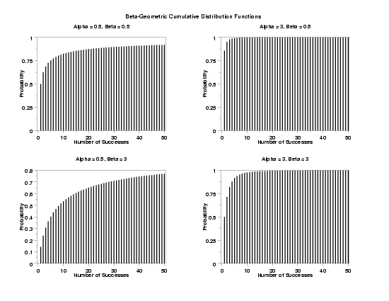
XLIMITS 0 50
XTIC OFFSET 0.5 0.5
LINE BLANK
SPIKE ON
SPIKE THICKNESS 0.3
.
TITLE CASE ASIS
LABEL CASE ASIS
X1LABEL Number of Successes
Y1LABEL Probability
.
MULTIPLOT 2 2
MULTIPLOT CORNER COORDINATES 0 0 100 95
MULTIPLOT SCALE FACTOR 2
.
TITLE Alpha = 0.5, Beta = 0.5
PLOT BGECDF(X,0.5,0.5) FOR X = 0 1 50
.
TITLE Alpha = 3, Beta = 0.5
PLOT BGECDF(X,3.0,0.5) FOR X = 0 1 50
.
TITLE Alpha = 0.5, Beta = 3
PLOT BGECDF(X,0.5,3.0) FOR X = 0 1 50
.
TITLE Alpha = 3, Beta = 3
PLOT BGECDF(X,3.0,3.0) FOR X = 0 1 50
.
END OF MULTIPLOT
.
CASE ASIS
JUSTIFICATION CENTER
MOVE 50 97
TEXT Beta-Geometric Cumulative Distribution Functions

Date created: 8/23/2006 |