TWO FACTOR PLOT

TWO FACTOR PLOT

Graphics Command

Given a response variable and associated variables containing laboratory id's and material id's, generate either a "laboratories within materials" or a "materials" within laboratories" plot.

This is essentially a run sequence plot sorted by the two factor variables.

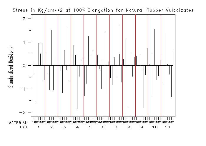
This plot is motivated by the desire to plot residuals for the "phase 3" analysis related to the ASTM E691 standard. The phase 3 analysis is a row-linear model for the data in a E691 study and was proposed by John Mandel (see the References below) as an additional step in the E691 analysis. In particular, Mandel recommended a plot of the standardized residuals from the row-linear model (specific plots for the h- and k-statistics are implemented with the H CONSISTENCY PLOT and K CONSISTENCY PLOT commands).

Although motivated by the E691 analysis, this plot can be used for any two factor data set from a full factorial design (i.e., all combinations of levels from the two factors are included). If there is replication within a cell, the mean of the replicates will be used.

TWO FACTOR PLOT <y> <labid> <matid>
                        <SUBSET/EXCEPT/FOR qualification>
where <y> is a response variable;
            <labid> is a variable that specifies the lab-id;
            <matid> is a variable that specifies the material-id;
and where the <SUBSET/EXCEPT/FOR qualification> is optional.

TWO FACTOR PLOT Y LABID MATID

If there is replication within the cells and you would like to plot something other than the mean value, you can use the LET CROSS TABULATE command. For example, to plot the standard deviations, do something like
SET LET CROSS TABULATE COLLAPSE
LET YSD = CROSS TABULATE SD Y X1 X2
LET X1D = CROSS TABULATE GROUP ONE X1 X2
LET X2D = CROSS TABULATE GROUP TWO X1 X2
TWO FACTOR PLOT YSD X1D X2D

There are two formats for the plots. By default, the values are plotted linearly. That is, given three laboratories and three materials, the x-axis is laid out as

 
LAB:  1  2  3  1  2  3  1  2  3
MAT:  1  1  1  2  2  2  3  3  3
X:    1  2  3  4  5  6  7  8  9
    

Alternatively, you can stack the lab values so that the x-axis is laid out as

 
LAB:  1  1  1
      2  2  2
      3  3  3
MAT:  1  2  3
X:    1  2  3
    

To specify the stacked alternative, enter the command

SET TWO FACTOR PLOT TYPE STACKED

To reset the line linear option, enter the command

SET TWO FACTOR PLOT TYPE DEFAULT

By default, the x-axis is defined by "laboratories within materials".

To define the x-axis as "materials within laboratories", enter the command

SET TWO FACTOR PLOT MATERIALS WITHIN LABORATORIES

To reset the default, enter

SET TWO FACTOR PLOT LABORATORIES WITHIN MATERIALS

We find it useful to generate both versions of the plot. Although the information being displayed is the same, different types of patterns may be clearer in one or the other of these plots.

For better separation between laboratories (or materials), you can enter the command
SET TWO FACTOR PLOT GAP <value>

where <value> is a non-negative integer. So in the above example,

SET TWO FACTOR PLOT GAP 1

yields

 
       LAB:  1  2  3  1  2  3  1  2  3
       MAT:  1  1  1  2  2  2  3  3  3
       X:    1  2  3  5  6  7  9 10 11
    

In some studies, the number of laboratories may be fairly large. In these cases, you may want to split the laboratories into multiple plots for better resolution.

To address this, the following commands were added

SET TWO FACTOR PLOT LABORATORY FIRST <value>
SET TWO FACTOR PLOT LABORATORY LAST <value>
SET TWO FACTOR PLOT MATERIAL FIRST <value>
SET TWO FACTOR PLOT MATERIAL LAST <value>


These commands allow you to specify the range of laboratories (or materials) to be displayed. Note that these commands limit you to contiguous ranges of laboratories or materials.

None

None

E691 INTERLAB	= Perform an interlaboratory analysis based on the E691 standard.
H CONSISTENCY PLOT	= Generate an h-consistency plot.
TWO WAY ROW PLOT	= Generate a plot based on Mandel's row linear analysis for two-way tables.

"Standard Practice for Conducting an Interlaboratory Study to Determine the Precision of a Test Method", ASTM International, 100 Barr Harbor Drive, PO BOX C700, West Conshohoceken, PA 19428-2959, USA.

Mandel (1994), "Analyzing Interlaboratory Data According to ASTM Standard E691", Quality and Statistics: Total Quality Management, ASTM STP 1209, Kowalewski, Ed., American Society for Testing and Materials, Philadelphia, PA 1994, pp. 59-70.

Mandel (1993), "Outliers in Interlaboratory Testing", Journal of Testing and Evaluation, Vol. 21, No. 2, pp. 132-135.

Mandel (1995), "Structure and Outliers in Interlaboratory Studies", Journal of Testing and Evaluation, Vol. 23, No. 5, pp. 364-369.

Mandel (1991), "Evaluation and Control of Measurements", Marcel Dekker, Inc.

Interlaboratory Studies

2015/5

 
. Step 1:   Read the data
.
dimension 40 columns
skip 25
read mandel7.dat y x1 x2
.
let nlab = unique x1
let nmat = unique x2
let ntot = nlab*nmat
.
variable label y Stress
variable label x1 Lab-ID
variable label x2 Rubber
let nlab = unique x1
let ncol = unique x2
.
. Step 2:   Define some default plot control settings
.
case asis
title case asis
title offset 2
label case asis
tic mark offset units screen
tic mark offset 3 3
.
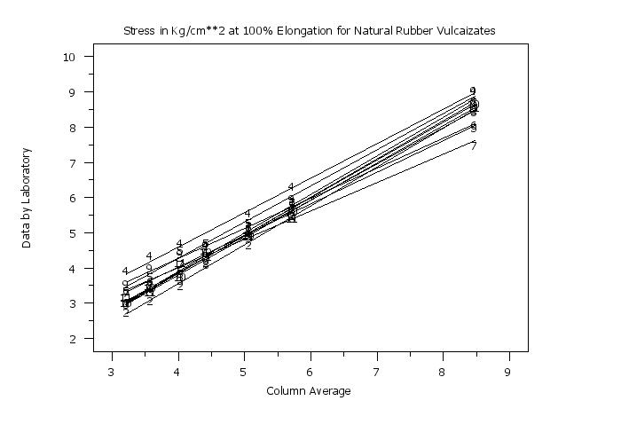
. Step 3:   Generate the two way row plot
.
x1label Column Average
character blank all
line dash all
loop for k = 1 1 nlab
    let kindex = (k-1)*2 + 1
    let plot character kindex = ^k
    let plot line      kindex = blank
end of loop
.
set two way plot factor label value
set two way plot factor decimal 4
set two way plot anova table on
set two way plot anova table decimals 4
set write decimals 4
title Stress in Kg/cm**2 at 100% Elongation for Natural Rubber Vulcaizates
y1label Data by Laboratory
.
two way row    plot y x1 x2
.
. Step 4:   Now generate the two factor plot of the residuals
.
skip 1
read dpst3f.dat labid matid junk1 junk2 junk3 resstd
skip 0
y1label Standardized Residuals
x1label Lab-ID/Rubber-ID
legend 1 MATERIAL:
legend 2 LAB:
legend 1 justification right
legend 2 justification right
legend 1 coordinates 14 15
legend 2 coordinates 14 12
legend 1 size 1.7
legend 2 size 1.7
.
x1label
x1tic mark label off
xlimits 1 ntot
major x1tic mark number ntot
minor x1tic mark number 0
x1tic mark offset 1 1
.
line blank
character blank
spike on
spike base 0
two factor plot resstd labid matid
line solid
drawdata 1 0 ntot 0
.
. Step 5:   Draw lines separating the labs and add tic labels
.           to identify labs/materials
.
let ycoorz = 16
let xcoor = 1
justification center
height 0.7
.
loop for k = 1 1 ntot
    moveds xcoor ycoorz
    let ktemp = mod(k-1,nmat) + 1
    text ^ktemp
    let xcoor = xcoor + 1
end of loop
.
height 1.5
let ycoorz = 12
let xcoor = (nmat/2)+0.5
line color red
line dash
loop for k = 1 1 nlab
    moveds xcoor ycoorz
    let ival = k
    text ^ival
    if k < nlab
       let xcoor2 = xcoor + (nmat/2)
       drawdsds xcoor2 20 xcoor2 90
    end of if
    let xcoor = xcoor + nmat
end of loop
line color black
line blank
    

The following output is generated

Parameters of Row-Linear Fit for Stress
-------------------------------------------------------------------------------------
                                                        Standard Error    Correlation
    Lab-ID         Height          Slope          RESSD       of Slope    Coefficient
-------------------------------------------------------------------------------------
    1.0000         4.9300         1.0909         0.1168         0.0268         0.9985
    2.0000         4.5957         1.0990         0.0851         0.0195         0.9992
    3.0000         4.8043         1.0613         0.1547         0.0355         0.9972
    4.0000         5.5200         0.9777         0.1818         0.0417         0.9955
    5.0000         5.0671         0.8575         0.1844         0.0423         0.9940
    6.0000         4.8657         0.8960         0.1289         0.0296         0.9973
    7.0000         4.7729         0.8063         0.1784         0.0409         0.9936
    8.0000         4.8543         1.0869         0.1006         0.0231         0.9989
    9.0000         5.2386         1.0304         0.2197         0.0504         0.9941
   10.0000         4.8571         1.0696         0.1045         0.0240         0.9987
   11.0000         4.8457         1.0244         0.1773         0.0407         0.9961
 
Standard Deviation of Slopes:                 0.1024
Pooled Standard Deviation of Fit:             0.1616
 
 
 
Column Averages
---------------------------
                     Column
      Rubber        Average
---------------------------
      1.0000         3.2291
      2.0000         3.5927
      3.0000         4.0418
      4.0000         4.4273
      5.0000         5.0791
      6.0000         5.7345
      7.0000         8.4827
 
Mean of Column Means:               4.9410
 
 
 
ANOVA Table for Row-Linear Fit
-----------------------------------------------------------------
                         Degrees of         Sum of           Mean
Source                      Freedom        Squares         Square
-----------------------------------------------------------------
Total                            76       216.8951         2.8539
Rows                             10         4.4471         0.4447
Column                            6       209.1488        34.8581
Error                            60         3.2991         0.0550
  Residuals                      50         1.3054         0.0261
  Slopes                         10         1.9937         0.1994
    Concurrence                   1         0.0496         0.0496
    Non-Concurrence               9         1.9441         0.2160