H CONSISTENCY PLOT
K CONSISTENCY PLOT
COCHRAN VARIANCE PLOT

H CONSISTENCY PLOT
K CONSISTENCY PLOT
COCHRAN VARIANCE PLOT

Graphics Command

Given a response variable and associated variables containing laboratory id's and material id's, generate a plot of one of the following versus material/laboratory:
1. h-consistency statistic
2. k-consistency statistic
3. Cochran variance outlier statistic

The h-consistency and k-consistency statistics are discussed in the ASTM E691 standard for interlaboratory analysis
"Standard Practice for Conducting an Interlaboratory Study to Determine the Precision of a Test Method", ASTM International, 100 Barr Harbor Drive, PO BOX C700, West Conshohoceken, PA 19428-2959, USA.

This standard addresses the situation where there are two factors (material and laboratory) and there is a full factorial balanced design (i.e., each combination of material and laboratory is run with an equal number of replications).

John Mandel has also discussed the h- and k-statistics in various publications (see the References section below).

The h-consistency statistic is a measure of the between laboratory consistency and is defined in the ASTM E691 standard as

\( h = d/s_{\tilde{x}} \)

with

d = cell deviation (cell average - average of cell averages)
\( s_{\tilde{x}} \) = standard deviations of cell averages

Essentially, h is standardized deviation from the grand averages. The critical value is computed as

\( hcv = \pm \frac{(p-1) t} {\sqrt{p(t^2 + p - 2)}} \)

where p denotes the number of laboratories and t denotes the percent point function of the t distribution with p - 2 degrees of freedom. The h consistency plot draws lines at the critical values corresponding to α = 0.5% (i.e., the 0.9975 and 0.0025 percent points of the t distribution). These are the values recommended in the E691 standard.

The k-consistency statistic is a measure of the within laboratory consistency and is defined in the ASTM E691 standard as

\( k = \frac{s} {s_r} \)

with

s = cell standard deviation
s_r = repeatability standard deviation

Essentially, k is the ratio of the cell standard devition to the pooled value. The critical value is computed as

\( kcv = \sqrt{\frac{p}{1 + (p-1) F}} \)

where p denotes the number of laboratories and F denotes the percent point function of the F distribution with (n-1) and (p-1)*(n-1) degrees of freedom. The k consistency plot draws a line at the critical value corresponding to α = 0.5% (i.e., the 0.995 percent point of the F distribution). This is the value recommended in the E691 standard.

The Cochran variance outlier test is a test for assessing the homogeneity of variances. It is essentially an outlier test for largest (or smallest) variance. Given k groups of data, some analyses assume the standard deviations (or equivalently, variances) are equal for the k groups. For example, the F test used in the one-factor analysis of variance problem can be sensitive to unequal standard deviations in the k levels of the factor.

The Levene and Bartlett tests are alternative tests widely used for assessing the homogeneity of variances in the one-factor (with k levels) case. Although the Cochran test has a similar purpose to the Levene and Bartlett tests, it tends to be used in a somewhat different context. The Levene and Bartlett test are used to assess overall homogeneity and are typically used in the context of deciding whether a specific test (e.g., an F test) is appropriate for a given set of data. These tests do not identify which variances are different. On the other hand, the Cochran variance outlier test tends to be used in the context of interlaboratory analysis. In this case, we are primarily interested in identifying laboratories that are "different". For example, a laboratory with an unusually large variance may indicate the need for close examination of that laboratory's practices.

Cochran's test is essentially an outlier test. Cochran's original test statistic is defined as

\( C = \frac{\mbox{largest} s_{i}^{2}} {\sum_{i=1}^{k}{s_{i}^{2}}} \)

That is, it is the ratio of the largest variance to the sum of the variances. This is an upper-tailed test for the maximum variance. The critical values can be computed from

\( C_{UL}(\alpha,n,k) = \frac{1} {1 + \frac{k-1}{FPPF(\alpha/k,(n-1),(k-1) (n-1))}} \)

where

CUL	=	the upper critical value (i.e., variance is an outlier if the test statistic is greater than CUL)
α	=	the significance level
n	=	the number of observations in each group
k	=	the number of groups
FPPF	=	the percent point function of the F distribution

Some comments on this test.

1. It assumes that the data in each group are normally distributed.

2. It assumes the sample sizes in each group are equal.

3. It tests for the maximum variance only (i.e., no test for the minimum variance).

't Lam (2009) has extended the Cochran test to support unequal sample sizes and tests for the minimum variance. He refers to this as the G statistic. Dataplot in fact generates the G statistic rather than the C statistic for this test. When the sample sizes are in fact equal, the G statistic for the maximum variance is equivalent to the Cochran C statistic.

The G statistic for the j-th group is

\( G_{j} = \frac{\nu_{j} s_{j}^{2}} {\sum_{i=1}^{k}{\nu_{i} s_{i}^{2}}} \)

where ν_i = n_i - 1 with n_i denoting the sample size of the i-th group.

The critical value for testing the maximum variance is

\( G_{UL}(\alpha,\nu_{j},\nu_{pool},k) = \frac{1} {1 + \frac{(\nu_{pool}/\nu_{j}) - 1} {FPPF(\alpha/k,\nu_{j},\nu_{pool}-\nu_{j})}} \)

where

\( \nu_{pool} \)	=	pooled degrees of freedom
	=	\( \sum_{i=1}^{k}{\nu_{i}} \)
\( \nu_{j} \)	=	the degrees of freedom corresponding to the maximum variance

Reject the null hypothesis that the maximum variance is an outlier if the test statistic is greater than the critical value.

The critical value for testing the minimum variance is

\( G_{LL}(\alpha,\nu_{j},\nu_{pool},k) = \frac{1} {1 + \frac{(\nu_{pool}/\nu_{j}) - 1} {FPPF(1 - \alpha/k,\nu_{j},\nu_{pool}-\nu_{j})}} \)

In this case, \( \nu_{j} \) corresponds to the minimum variance. Reject the null hypothesis that the minimum variance is an outlier if the test statistic is less than the critical value.

A two-sided test can also be performed. Just use α/2 in place of α in the above formulas. Although the 't Lam article provides a method for determining whether the maximum or minimum variance is more extreme, Dataplot will simply return the test statistic and critical values for both the maximum and the minimum cases.

Note that with the G statistic, we are actually testing for the maximum (or minimum) value of the G statistic rather than the maximum (or minimum) variance. If the sample sizes are equal (or at least approximately equal), this should be equivalent. However, if there is a large difference in sample sizes, this may not be the case. That is, we are testing the maximum \( \nu_{j} s_{j}^{2} \) rather than the maximum \( s_{j}^{2} \).

H CONSISTENCY PLOT <y> <labid> <matid>
                        <SUBSET/EXCEPT/FOR qualification>
where <y> is a response variable;
            <labid> is a variable that specifies the lab-id;
            <matid> is a variable that specifies the material-id;
and where the <SUBSET/EXCEPT/FOR qualification> is optional.

This syntax plots the h-consistency statistic. The variables must all be of equal length.

K CONSISTENCY PLOT <y> <labid> <matid>
                        <SUBSET/EXCEPT/FOR qualification>
where <y> is a response variable;
            <labid> is a variable that specifies the lab-id;
            <matid> is a variable that specifies the material-id;
and where the <SUBSET/EXCEPT/FOR qualification> is optional.

This syntax plots the k-consistency statistic. The variables must all be of equal length.

COCHRAN VARIANCE PLOT <y> <labid> <matid>
                        <SUBSET/EXCEPT/FOR qualification> where <y> is a response variable;
<labid> is a variable that specifies the lab-id;
<matid> is a variable that specifies the material-id;
and where the <SUBSET/EXCEPT/FOR qualification> is optional.

This syntax plots the Cochran variance statistic. The variables must all be of equal length.

H CONSISTENCY PLOT Y LABID MATID
K CONSISTENCY PLOT Y LABID MATID
COCHRAN VARIANCE PLOT Y LABID MATID
H CONSISTENCY PLOT Y LABID MATID SUBSET MATID > 2

There are two formats for the plots. By default, the values are plotted linearly. That is, given three laboratories and three materials, the x-axis is laid out as

 
LAB:  1  2  3  1  2  3  1  2  3
MAT:  1  1  1  2  2  2  3  3  3
X:    1  2  3  4  5  6  7  8  9
    

Alternatively, you can stack the lab values so that the x-axis is laid out as

 
LAB:  1  1  1
      2  2  2
      3  3  3
MAT:  1  2  3
X:    1  2  3
    

To specify the stacked alternative, enter the command

SET H CONSISTENCY PLOT TYPE STACKED

To reset the line linear option, enter the command

SET H CONSISTENCY PLOT TYPE DEFAULT

By default, the x-axis is defined by "laboratories within materials".

To defined the x-axis as "materials within laboratories", enter the command

SET H CONSISTENCY PLOT MATERIALS WITHIN LABORATORIES

To reset the default, enter

SET H CONSISTENCY PLOT LABORATORIES WITHIN MATERIALS

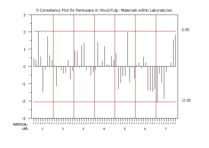
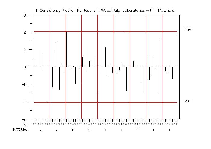
We find it useful to generate both versions of the plot. Although the information being displayed is the same, different types of patterns may be clearer in one or the other of these plots.

For better separation between laboratories (or materials), you can enter the command
SET H CONSISTENCY PLOT GAP <value>

where <value> is a non-negative integer. So in the above example,

SET H CONSISTENCY PLOT GAP 1

yields

LAB:  1  2  3  1  2  3  1  2  3
MAT:  1  1  1  2  2  2  3  3  3
X:    1  2  3  5  6  7  9 10 11
    

In some studies, the number of laboratories may be fairly large. In these cases, you may want to split the laboratories into multiple plots for better resolution. However, you want to include all laboratories and materials in the computation of the h- and k-consistency statistics. Simply using the SUBSET clause to specify which laboratories (or materials) are excluded from the plot will also exclude them from the computation of the statistics.

To address this, the following commands were added

SET H CONSISTENCY PLOT LABORATORY FIRST <value>
SET H CONSISTENCY PLOT LABORATORY LAST <value>
SET H CONSISTENCY PLOT MATERIAL FIRST <value>
SET H CONSISTENCY PLOT MATERIAL LAST <value>


These commands allow you to specify the range of laboratories (or materials) to be displayed while still using the full set in computing the statistics. Note that these commands limit you to contiguous ranges of laboratories or materials.

In some sense, these plots are used to identify outliers. However, Mandel has emphasized that the purpose is primarily identification of systematic patterns rather than rejection of outlying laboratories.

That is, if there are laboratories that are systematically higher or systematically lower than the others, then the test protocol should be carefully examined. Although rejection may be warranted in the case of an obvious error, the real purpose is to improve the underlying measurement process. That is, does the method itself produce consist results with different laboratories? Was the specification of the method clear enough so that different laboratories imnplemented it in a consistent manner?

The 2023 version of the E691 standard was updated to support unbalanced data. Note that the E691 standard still recommends that the study be designed as a balanced design. Support for unbalanced data is incorporated so that if a laboratory has a bad measurement, that laboratory does not have to be removed from the study.

The 2024/05 version updated the E691 command to support unbalanced data. The formulas for the unbalanced data are given in section A2 of the 2023 version of the standard and are not given here.

None

The various SET H CONSISTENCY PLOT commands can also be given as SET K CONSISTENCY PLOT or SET COCHRAN VARIANCE PLOT. Regardless of which is used, the SET commands will apply to all threee variations of the plot.

H CONSISTENCY STATISTIC	= Compute the h-consistency statistic.
K CONSISTENCY STATISTIC	= Compute the k-consistency statistic.
COCHRAN VARIANCE OUTLIER TEST	= Perform Cochran's variance outlier test.
E691 INTERLAB	= Perform an interlaboratory analysis based on the E691 standard.
TWO FACTOR PLOT	= Generate a run sequence plot with two factor variables.
TWO WAY ROW PLOT	= Generate a plot based on Mandel's row linear analysis for two-way tables.

"Standard Practice for Conducting an Interlaboratory Study to Determine the Precision of a Test Method", ASTM International, 100 Barr Harbor Drive, PO BOX C700, West Conshohoceken, PA 19428-2959, USA.

Mandel (1994), "Analyzing Interlaboratory Data According to ASTM Standard E691", Quality and Statistics: Total Quality Management, ASTM STP 1209, Kowalewski, Ed., American Society for Testing and Materials, Philadelphia, PA 1994, pp. 59-70.

Mandel (1993), "Outliers in Interlaboratory Testing", Journal of Testing and Evaluation, Vol. 21, No. 2, pp. 132-135.

Mandel (1995), "Structure and Outliers in Interlaboratory Studies", Journal of Testing and Evaluation, Vol. 23, No. 5, pp. 364-369.

Mandel (1991), "Evaluation and Control of Measurements", Marcel Dekker, Inc..

Interlaboratory Studies

2015/05
2024/05: H CONSISTENCY PLOT and K CONSISTENCY PLOT updated to support unbalanced data

 
. Step 1:   Read the data
.
skip 25
read mandel6.dat y labid matid
.
. Step 2:   Default plot control settings
.
case asis
label case asis
tic mark label case asis
title case asis
title offset 2
.
. Step 3:   Plot options
.
let nlab = unique labid
let nmat = unique matid
let ntot = nlab*nmat
.
xlimits 1 ntot
major x1tic mark number ntot
minor x1tic mark number 0
x1tic mark offset 1 1
x1tic mark label off
legend 1 MATERIAL:
legend 2 LAB:
legend 1 justification right
legend 2 justification right
legend 1 coordinates 14 12
legend 2 coordinates 14 15
legend 1 size 1.7
legend 2 size 1.7
spike on
spike base 0
line blank solid solid solid
line color black black red red
.
. Step 4:   Generate the plot
.
title h Consistency Plot for  Pentosans in Wood Pulp: Laboratories within Materials
h consistency plot y labid matid
.
just left
let atemp = round(hcv,2)
movesd 87 atemp
text ^atemp
let atemp = -atemp
movesd 87 atemp
text ^atemp
.
let ycoorz = 16
let xcoor = 1
justification center
height 1.0
.
loop for k = 1 1 ntot
    moveds xcoor ycoorz
    let ktemp = mod(k-1,nlab) + 1
    text ^ktemp
    let xcoor = xcoor + 1
end of loop
.
height 1.5
let ycoorz = 12
let xcoor = (nlab/2)+0.5
line color red
line dash
loop for k = 1 1 nmat
    moveds xcoor ycoorz
    let ival = k
    text ^ival
    if k < nmat
       let xcoor2 = xcoor + (nlab/2)
       drawdsds xcoor2 20 xcoor2 90
    end of if
    let xcoor = xcoor + nlab
end of loop
line color black
line blank
    

 
. Step 1:   Read the data
.
skip 25
read mandel6.dat y labid matid
.
. Step 2:   Default plot control settings
.
case asis
label case asis
tic mark label case asis
title case asis
title offset 2
.
. Step 3:   Plot options
.
let nlab = unique labid
let nmat = unique matid
let ntot = nlab*nmat
.
set h consistency plot materials within Laboratories
xlimits 1 ntot
major x1tic mark number ntot
minor x1tic mark number 0
x1tic mark offset 1 1
x1tic mark label off
legend 1 MATERIAL:
legend 2 LAB:
legend 1 justification right
legend 2 justification right
legend 1 coordinates 14 15
legend 2 coordinates 14 12
legend 1 size 1.7
legend 2 size 1.7
spike on
spike base 0
line blank solid solid solid
line color black black red red
.
. Step 4:   Generate the plot
.
title h Consistency Plot for Pentosans in Wood Pulp: Materials within Laboratories
h consistency plot y labid matid
.
just left
let atemp = round(hcv,2)
movesd 87 atemp
text ^atemp
let atemp = -atemp
movesd 87 atemp
text ^atemp
.
let ycoorz = 16
let xcoor = 1
justification center
height 1.0
.
loop for k = 1 1 ntot
    moveds xcoor ycoorz
    let ktemp = mod(k-1,nmat) + 1
    text ^ktemp
    let xcoor = xcoor + 1
end of loop
.
height 1.5
let ycoorz = 12
let xcoor = (nmat/2)+0.5
line color red
line dash
loop for k = 1 1 nlab
    moveds xcoor ycoorz
    let ival = k
    text ^ival
    if k < nlab
       let xcoor2 = xcoor + (nmat/2)
       drawdsds xcoor2 20 xcoor2 90
    end of if
    let xcoor = xcoor + nmat
end of loop
line color black
line blank