COCHRAN VARIANCE OUTLIER TEST

COCHRAN VARIANCE OUTLIER TEST

Analysis Command

Perform Cochran's variance outlier test to assess the homogeneity of variances in the one-factor case.

Given k groups of data, some analyses assume the standard deviations (or equivalently, variances) are equal for the k groups. For example, the F test used in the one-factor analysis of variance problem can be sensitive to unequal standard deviations in the k levels of the factor.

The Levene and Bartlett tests are widely used for assessing the homogeneity of variances in the one-factor (with k levels) case. The Cochran variance outlier test is another alternative for assessing the homogeneity of variances.

Although the Cochran test has a similar purpose to the Levene and Bartlett tests, it tends to be used in a somewhat different context. The Levene and Bartlett test are used to assess overall homogeneity and are typically used in the context of deciding whether a specific test (e.g., an F test) is appropriate for a given set of data. These tests do not identify which variances are different. On the other hand, the Cochran variance outlier test tends to be used in the context of proficiency testing. In this case, we are primarily interested in identifying laboratories that are "different". For example, a laboratory with an unusually large variance may indicate the need for close examination of that laboratory's practices.

Cochran's test is essentially an outlier test. Cochran's original test statistic is defined as

\( C = \frac{\mbox{largest} s_{i}^{2}} {\sum_{i=1}^{k}{s_{i}^{2}}} \)

That is, it is the ratio of the largest variance to the sum of the variances. This is an upper-tailed test for the maximum variance. The critical values can be computed from

\( C_{UL}(\alpha,n,k) = \frac{1} {1 + \frac{k-1}{FPPF(\alpha/k,(n-1),(k-1) (n-1))}} \)

where

CUL	=	the upper critical value (i.e., variance is an outlier if the test statistic is greater than CUL)
α	=	the significance level
n	=	the number of observations in each group
k	=	the number of groups
FPPF	=	the percent point function of the F distribution

Some comments on this test.

1. It assumes that the data in each group are normally distributed.

2. It assumes the sample sizes in each group are equal.

3. It tests for the maximum variance only (i.e., no test for the minimum variance).

't Lam (2009) has extended the Cochran test to support unequal sample sizes and tests for the minimum variance. He refers to this as the G statistic. Dataplot in fact generates the G statistic rather than the C statistic for this test. When the sample sizes are in fact equal, the G statistic for the maximum variance is equivalent to the Cochran C statistic.

The G statistic for the j-th group is

\( G_{j} = \frac{\nu_{j} s_{j}^{2}} {\sum_{i=1}^{k}{\nu_{i} s_{i}^{2}}} \)

where ν_i = n_i - 1 with n_i denoting the sample size of the i-th group.

The critical value for testing the maximum variance is

\( G_{UL}(\alpha,\nu_{j},\nu_{pool},k) = \frac{1} {1 + \frac{(\nu_{pool}/\nu_{j}) - 1} {FPPF(\alpha/k,\nu_{j},\nu_{pool}-\nu_{j})}} \)

where

\( \nu_{pool} \)	=	pooled degrees of freedom
	=	\( \sum_{i=1}^{k}{\nu_{i}} \)
\( \nu_{j} \)	=	the degrees of freedom corresponding to the maximum variance

Reject the null hypothesis that the maximum variance is an outlier if the test statistic is greater than the critical value.

The critical value for testing the minimum variance is

\( G_{LL}(\alpha,\nu_{j},\nu_{pool},k) = \frac{1} {1 + \frac{(\nu_{pool}/\nu_{j}) - 1} {FPPF(1 - \alpha/k,\nu_{j},\nu_{pool}-\nu_{j})}} \)

In this case, \( \nu_{j} \) corresponds to the minimum variance. Reject the null hypothesis that the minimum variance is an outlier if the test statistic is less than the critical value.

A two-sided test can also be performed. Just use α/2 in place of α in the above formulas. Although the 't Lam article provides a method for determining whether the maximum or minimum variance is more extreme, Dataplot will simply return the test statistic and critical values for both the maximum and the minimum cases.

Note that with the G statistic, we are actually testing for the maximum (or minimum) value of the G statistic rather than the maximum (or minimum) variance. If the sample sizes are equal (or at least approximately equal), this should be equivalent. However, if there is a large difference in sample sizes, this may not be the case. That is, we are testing the maximum \( \nu_{j} s_{j}^{2} \) rather than the maximum \( s_{j}^{2} \).

If there are potentially multiple outliers in the variances, the recommended procedure is to perform the test sequentially until all outlying variances are removed. That is, if the test indicates the maximum variance is an outlier, remove that group of data and perform the test again. Repeat until the test indicates that

COCHRAN VARIANCE OUTLIER TEST <y> <tag>
                        <SUBSET/EXCEPT/FOR qualification>
where <y> is a response variable;
            <tag> is a factor identifier variable;
and where the <SUBSET/EXCEPT/FOR qualification> is optional.

This syntax computes the test for the maximum variance.

COCHRAN MINIMUM VARIANCE OUTLIER TEST <y> <tag>
                        <SUBSET/EXCEPT/FOR qualification>
where <y> is a response variable;
            <tag> is a factor identifier variable;
and where the <SUBSET/EXCEPT/FOR qualification> is optional.

This syntax computes the test for the minimum variance.

COCHRAN TWO-SIDED VARIANCE OUTLIER TEST <y> <tag>
                        <SUBSET/EXCEPT/FOR qualification>
where <y> is a response variable;
            <tag> is a factor identifier variable;
and where the <SUBSET/EXCEPT/FOR qualification> is optional.

This syntax computes the two-sided test (i.e., both the minimum and maximum variance).

MULTIPLE COCHRAN VARIANCE OUTLIER TEST <y1> ... <yk>
                        <SUBSET/EXCEPT/FOR qualification>
where <y1> ... <yk> is a list of two to 30 response variables;
and where the <SUBSET/EXCEPT/FOR qualification> is optional.

This syntax computes the test for the maximum variance.

MULTIPLE COCHRAN MINIMUM VARIANCE OUTLIER TEST <y1> ... <yk>
                        <SUBSET/EXCEPT/FOR qualification>
where <y1> ... <yk> is a list of two to 30 response variables;
and where the <SUBSET/EXCEPT/FOR qualification> is optional.

This syntax computes the test for the minimum variance.

MULTIPLE COCHRAN TWO-SIDED VARIANCE OUTLIER TEST <y1> ... <yk>
                        <SUBSET/EXCEPT/FOR qualification>
where <y1> ... <yk> is a list of two to 30 response variables;
and where the <SUBSET/EXCEPT/FOR qualification> is optional.

This syntax computes the two-sided test.

COCHRAN VARIANCE OUTLIER TEST Y X
COCHRAN VARIANCE OUTLIER TEST Y X SUBSET X <> 5
COCHRAN MINIMUM VARIANCE OUTLIER TEST Y X
COCHRAN TWO-SIDED VARIANCE OUTLIER TEST Y X

The following parameters are created automatically by this command

STATVAL	=	value of test statistic for either the maximum or the minimum case
STATCDF	=	CDF of the test statistic for either the maximum or the minimum case
PVALUE	=	p-value of the test statistic for either the maximum or the minimum case
STATVALU	=	value of test statistic for the maximum variance for the two-sided test
STATVALL	=	value of test statistic for the minimum variance for the two-sided test
CUTOF001	=	the 0.1% critical value
CUTOF005	=	the 0.5% critical value
CUTOFF01	=	the 1% critical value
CUTOF025	=	the 2.5% critical value
CUTOFF05	=	the 5% critical value
CUTOFF10	=	the 10% critical value
CUTOFF25	=	the 25% critical value
CUTOFF50	=	the 50% critical value
CUTOFF75	=	the 75% critical value
CUTOFF90	=	the 90% critical value
CUTOFF95	=	the 95% critical value
CUTOF975	=	the 97.5% critical value
CUTOFF99	=	the 99% critical value
CUTOF995	=	the 99.5% critical value
CUTOF999	=	the 99.9% critical value

P-values are truncated at a minimum of 0.001 and a maximum of 99.999. P-values and CDF statistics are not currently computed for the two-sided case.

In proficiency testing, John Mandel's k consistency statistic has been used (specifically, the ASTM E-691 standard) to identify laboratories with excessively large variances.

The ISO 5725 standard proposes Cochran's variance outlier test as an alternative to Mandel's k consistency statistic.

The following statistics are also supported:

LET C = COCHRAN VARIANCE OUTLIER TEST Y X
LET CV95 = COCHRAN VARIANCE OUTLIER CV95 Y X
LET CV99 = COCHRAN VARIANCE OUTLIER CV99 Y X
LET CCDF = COCHRAN VARIANCE OUTLIER CDF Y X
LET CPVAL = COCHRAN VARIANCE OUTLIER PVALUE Y X
LET CM = COCHRAN MINIMUM VARIANCE OUTLIER TEST Y X
LET CMV05 = COCHRAN MINIMUM VARIANCE OUTLIER CV05 Y X
LET CMV01 = COCHRAN MINIMUM VARIANCE OUTLIER CV01 Y X
LET CMCDF = COCHRAN MINIMUM VARIANCE OUTLIER CDF Y X
LET CMPVAL = COCHRAN MINIMUM VARIANCE OUTLIER PVALUE Y X


Enter HELP STATISTICS to see what commands can use these statistics.

If MIMIMUM or TWO-SIDED is not specified on the command, a test will be performed for the maximum variance.

COCHRAN VARIANCE OUTLIER is a synonym for COCHRAN VARIANCE OUTLIER TEST

LEVENE TEST	= Compute Levene's test for equal variances.
BARTLETT TEST	= Compute Bartlett's test for equal variances.
F TEST	= Performs a two-sample F test for equal variances.
VARIANCE PLOT	= Plot variances against group-id's.

W.G. Cochran (1941), "The distribution of the largest of a set of estimated variances as a fraction of their total," Annals of Human Genetics, (London) 11(1), pp. 47–52.

Ruben U.E. 't Lam (2010), "Scrutiny of Variance Results for Outliers: Cochran's Test Optimized", Analytica Chimica ACTA, Vol. 659, No. 1-2, pp. 68-84.

Kanji (2006), "100 Statistical Tests", SAGE Publications, p. 75.

ISO Standard 5725–2:1994, “Accuracy (trueness and precision) of measurement methods and results – Part 2: Basic method for the determination of repeatability and reproducibility of a standard measurement method”, International Organization for Standardization, Geneva, Switzerland, 1994.

Proficiency Tests

2015/04

 
. Step 1:   Read the data
.
dimension 40 columns
skip 25
read gear.dat y x
set write decimals 5
.
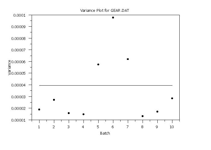
. Step 2:   Generate a variance plot
.
label case asis
title case asis
title offset 2
xlimits 1 10
major x1tic mark number 10
x1tic mark offset 0.5 0.5
x1label Batch
y1label Variance
line blank solid
character circle blank
character hw 1 0.75
character fill on
title Variance Plot for GEAR.DAT
variance plot y x
.
. Step 2:   Perform the test
.
.
cochran variance outlier test y x
let c     = cochran variance outlier test y x
let cv95  = cochran variance outlier cv95 y x
let cv99  = cochran variance outlier cv99 y x
let ccdf  = cochran variance outlier cdf y x
let cpval = cochran variance outlier pvalue y x
print c cv95 cv99 ccdf cpval
cochran minimum variance outlier test y x
let cm     = cochran minimum variance outlier test y x
let cmv05  = cochran minimum variance outlier cv05 y x
let cmv01  = cochran minimum variance outlier cv01 y x
let cmcdf  = cochran minimum variance outlier cdf y x
let cmpval = cochran minimum variance outlier pvalue y x
print cm cmv05 cmv01 cmcdf cmpval
cochran two-sided variance outlier test y x
    

The following output is generated



            Cochran Variance Outlier Test
 
Response Variable: Y
Group-ID Variable: X
 
H0: Largest Variance is Not an Outlier
Ha: Largest Variance is an Outlier
 
Summary Statistics:
Total Number of Observations:            100
Number of Groups:                        10
Number of Groups with Positive Variance: 10
Group with Largest Variance:             6
Largest Variance:                        0.00010
Sum of Variance:                         0.00317
 
Cochran Test Statistic Value:            0.27713
CDF of Test Statistic:                   0.98790
P-Value:                                 0.01210
 
 
Percent Points of the Reference Distribution
-----------------------------------
  Percent Point               Value
-----------------------------------
            0.1    =        0.15970
            0.5    =        0.15983
            1.0    =        0.16000
            2.5    =        0.16051
            5.0    =        0.16137
           10.0    =        0.16315
           25.0    =        0.16905
           50.0    =        0.18164
           75.0    =        0.20180
           90.0    =        0.22643
           95.0    =        0.24388
           97.5    =        0.26050
           99.0    =        0.28139
           99.5    =        0.29648
           99.9    =        0.32953
 
Conclusions (Upper 1-Tailed Test)
----------------------------------------------
  Alpha    CDF   Critical Value     Conclusion
----------------------------------------------
    10%    90%          0.22643      Reject H0
     5%    95%          0.24388      Reject H0
   2.5%  97.5%          0.26050      Reject H0
     1%    99%          0.28139      Accept H0
 

 PARAMETERS AND CONSTANTS--

    C       --        0.27713
    CV95    --        0.24388
    CV99    --        0.28139
    CCDF    --        0.98790
    CPVAL   --        0.01210
 
            Cochran Variance Outlier Test
 
Response Variable: Y
Group-ID Variable: X
 
H0: Smallest Variance is Not an Outlier
Ha: Smallest Variance is an Outlier
 
Summary Statistics:
Total Number of Observations:            100
Number of Groups:                        10
Number of Groups with Positive Variance: 10
Group with Smallest Variance:            8
Smallest Variance:                       0.00001
Sum of Variance:                         0.00317
 
Cochran Test Statistic Value:            0.03730
CDF of Test Statistic:                   0.44640
P-Value:                                 0.44640
 
 
Percent Points of the Reference Distribution
-----------------------------------
  Percent Point               Value
-----------------------------------
            0.1    =        0.00779
            0.5    =        0.01144
            1.0    =        0.01355
            2.5    =        0.01702
            5.0    =        0.02033
           10.0    =        0.02442
           25.0    =        0.03147
           50.0    =        0.03861
           75.0    =        0.04383
           90.0    =        0.04650
           95.0    =        0.04734
           97.5    =        0.04775
           99.0    =        0.04800
           99.5    =        0.04808
           99.9    =        0.04814
 
Conclusions (Lower 1-Tailed Test)
----------------------------------------------
  Alpha    CDF   Critical Value     Conclusion
----------------------------------------------
     1%     1%          0.01355      Accept H0
   2.5%   2.5%          0.01702      Accept H0
     5%     5%          0.02033      Accept H0
    10%    10%          0.02442      Accept H0
 

 PARAMETERS AND CONSTANTS--

    CM      --        0.03730
    CMV05   --        0.02033
    CMV01   --        0.01355
    CMCDF   --        0.44640
    CMPVAL  --        0.44640
 
            Cochran Variance Outlier Test
 
Response Variable: Y
Group-ID Variable: X
 
H0: Extreme Variance is Not an Outlier
Ha: Extreme Variance is an Outlier
 
Summary Statistics:
Total Number of Observations:            100
Number of Groups:                        10
Number of Groups with Positive Variance: 10
Group with Largest Variance:             6
Largest Variance:                        0.00010
Sum of Variance:                         0.00317
 
Cochran Test Statistic Value (upper):    0.27713
Cochran Test Statistic Value (lower):    0.03730
 
 
Conclusions (Two-Tailed Test)
-----------------------------------------------------------------------
          Significance            Lower            Upper
  Alpha          Level   Critical Value   Critical Value     Conclusion
-----------------------------------------------------------------------
    10%            90%          0.02033          0.24388      Reject H0
     5%            95%          0.01702          0.26050      Reject H0
     1%            99%          0.01144          0.29648      Accept H0