I PLOT

I PLOT

Graphics Command

Generates an I plot.

Given a response variable and a group-id variable, the I plot is used to plot a location value, a lower extreme value, and an upper extreme value for each group. The default is to use the median for the location and the minimum and maximum values as the extreme points (alternatives will be discussed below).

An I plot is used in two ways:

1. As a graphical data analysis technique (similar to the box plot, but simpler) for determining if differences exist between the various levels of a 1-factor model. It is a graphical alternative to 1-factor ANOVA.

2. As an uncertainty chart in which the analyst wishes to plot estimated values of a certain quantity and to also illustrate the uncertainty bars associated with each estimate. In such case, a given value of the horizontal axis variable is typically accompanied by exactly 3 values for the vertical axis variable:
   1. the estimate - the uncertainty;
   2. the estimate;
   3. the estimate + the uncertainty.

For both applications, the resulting plot is similar in appearance. Namely, a target value which typically appears as an X, a vertical bar with small horizontal bars at the extremes (hence the name "I plot").

The I plot has five components (characters and lines) which can be individually controlled. These components are:

1. the maximum (or upper extreme value)
2. the median (or other location value)
3. the minimum (or lower extreme value)
4. the line between the median (location value) and the maximum (upper extreme)
5. the line between the median (location value) and the minimum (lower extreme)

For the default I plot, the I PLOT command can be preceded by the following two commands:

CHARACTERS I PLOT
LINES I PLOT


With these commands, the first three lines are set to blank and lines four and five are set blank. The second character is set to "X", characters one and three are set to "-", and characters four and five are set to blank. After the I plot is formed, the analyst should redefine plot characters and lines via the usual CHARACTERS and LINES commands.

As mentioned above, the I plot can use location statistics other than the median. Specifically, you can use the MEAN I PLOT, MIDMEAN I PLOT, MIDRANGE I PLOT, TRIMMED MEAN I PLOT, and BIWEIGHT I PLOT to specify the mean, midmean, midrange, trimmed mean, and biweight location, respectively.

This plot is also useful for displaying confidence intervals as well as other types of intervals. The following are currently supported:

1. mean confidence limits
2. trimmed mean confidence limits
3. median confidence limits
4. quantile confidence limits
5. biweight confidence limits
6. one standard error (mean ± \(s/\sqrt{n}\))
7. two standard error (mean ± \(2s/\sqrt{n}i\))
8. one standard deviation (mean ± s)
9. two standard deviation (mean ± 2s)
10. standard deviation confidence limits
11. coefficient of variation confidence limits
12. coefficient of dispersion confidence limits
13. difference of means confidence limits
14. normal tolerance limits
15. normal prediction limits
16. Agresti Coull limits (for binomial proportions)
17. difference of proportions confidence limits
18. correlation confidence limits
19. ratio of means confidence limits

<stat> I PLOT <y> <x>             <SUBSET/EXCEPT/FOR qualification>
where <stat> is MEDIAN, MEAN, MIDMEAN, MIDRANGE, BIWEIGHT,
                       or TRIMMED MEAN;
            <y> is the response (= dependent) variable;
            <x> is the horizontal axis (= independent) variable;
and where the <SUBSET/EXCEPT/FOR qualification> is optional.

For this syntax, the extreme values will be the minimum and maximum values. If <stat> is omitted, the location statistic will be the median.

<stat> PLOT <y> <x>             <SUBSET/EXCEPT/FOR qualification>
where <stat> is one of:
                       MEAN CONFIDENCE LIMIT
                       TRIMMED MEAN CONFIDENCE LIMIT
                       MEDIAN CONFIDENCE LIMIT
                       QUANTILE CONFIDENCE LIMIT
                       BIWEIGHT CONFIDENCE LIMIT
                       STANDARD DEVIATION CONFIDENCE LIMIT
                       NORMAL TOLERANCE LIMIT
                       NORMAL PREDICTION LIMIT
                       AGRESTI COULL LIMIT
                       ONE STANDARD ERROR
                       TWO STANDARD ERROR
                       ONE STANDARD DEVIATION
                       TWO STANDARD DEVIATIONS
                       STANDARD DEVIATION CONFIDENCE LIMIT
                       COEFFICIENT OF VARIATION CONFIDENCE LIMIT
                       COEFFICIENT OF DISPERSION CONFIDENCE LIMIT
            <y> is the response (= dependent) variable;
            <x> is the horizontal axis (= independent) variable;
and where the <SUBSET/EXCEPT/FOR qualification> is optional.

For this syntax, the extreme values will be the lower and upper bounds of the appropriate limits.

<stat> PLOT <y1> <y2> <x>             <SUBSET/EXCEPT/FOR qualification>
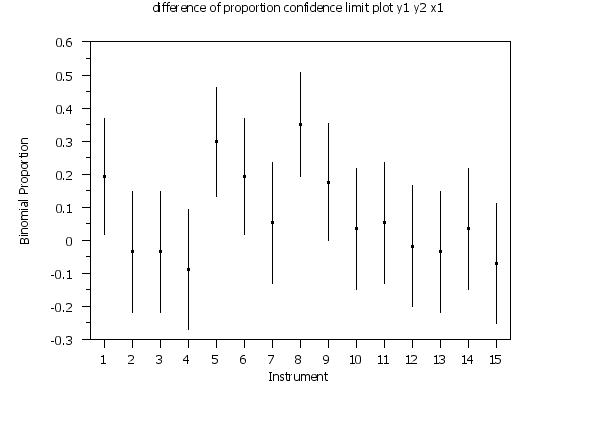
where <stat> is one of:
                       DIFFERENCE OF MEANS CONFIDENCE LIMIT
                       DIFFERENCE OF PROPORTIONS CONFIDENCE LIMIT
                       RATIO OF MEANS CONFIDENCE LIMIT
                       CORRELATION CONFIDENCE LIMIT
            <y1> is the first response (= dependent) variable;
            <y2> is the second response (= dependent) variable;
            <x> is the horizontal axis (= independent) variable;
and where the <SUBSET/EXCEPT/FOR qualification> is optional.

This is similar to Syntax 2 except that there are two response variables instead of one.

MULTIPLE <stat> PLOT <y1> ... <yk>
                        <SUBSET/EXCEPT/FOR qualification>
where <stat> is one of:
                        MEDIAN I
                        MEAN I
                        MIDMEAN I
                        MIDRANGE I
                        BIWEIGHT I
                        TRIMMED MEAN I
                        MEAN CONFIDENCE LIMIT
                        TRIMMED MEAN CONFIDENCE LIMIT
                        MEDIAN CONFIDENCE LIMIT
                        QUANTILE CONFIDENCE LIMIT
                        BIWEIGHT CONFIDENCE LIMIT
                        STANDARD DEVIATION CONFIDENCE LIMIT
                        COEFFICIENT OF VARIATION CONFIDENCE LIMIT
                        COEFFICIENT OF DISPERSION CONFIDENCE LIMIT
                        NORMAL TOLERANCE LIMIT
                        NORMAL PREDICTION LIMIT
                        AGRESTI COULL LIMIT
                        ONE STANDARD ERROR
                        TWO STANDARD ERROR
                        ONE STANDARD DEVIATION
                        TWO STANDARD DEVIATION
            <y1> ... <yk> is a list of up to k response variables;
and where the <SUBSET/EXCEPT/FOR qualification> is optional.

This syntax is useful when the data for each group is stored in separate response variables. Up to 30 response variables may be specified.

Note that the syntax

MULTIPLE I PLOT Y1 TO Y4

is supported. This is equivalent to

MULTIPLE I PLOT Y1 Y2 Y3 Y4

REPLICATED <stat> PLOT <y> <x1> ... <xk>
                        <SUBSET/EXCEPT/FOR qualification>
where <stat> is one of the variants listed for Syntax 4;
            <y> is the response variable;
            <x1> ... <xk> is a list of up to k group-id variables;
and where the <SUBSET/EXCEPT/FOR qualification> is optional.

This syntax performs a cross-tabulation of <x1> ... <xk> and generates an i plot (on the same graph) for each unique combination of cross-tabulated values. For example, if X1 has 3 levels and X2 has 2 levels, there will be a total of 6 i plots generated. Up to six group-id variables can be specified.

Note that the syntax

REPLICATED I PLOT Y X1 TO X4

is supported. This is equivalent to

REPLICATED I PLOT Y X1 X2 X3 X4

In this syntax, all i plots are drawn with the sampe plot attributes.

As an example of how the x-coordinates are determined, assume we have 3 levels for X1 and 2 levels for X2. The x-coordinates will be

X1	X2	X-COORDINATE
1	1	1
1	2	2
2	1	3
2	2	4
3	1	5
3	2	6

<stat> PLOT <y> <x1> <x2>
                        <SUBSET/EXCEPT/FOR qualification>
where <stat> is one of the variants listed for Syntax 4;
            <y> is the response variable;
            <x1> is the first group-id variable;
            <x2> is the second group-id variable;
and where the <SUBSET/EXCEPT/FOR qualification> is optional.

This syntax is similar to syntax 5. However, it has the following distinctions:

1. There must be exactly two group-id variables and the word REPLICATION is omitted from the command.

2. The groups in the second group-id variable are drawn with different attributes.

3. The x-coordinates are generated to emphasize the comparisons between the groups for each level of the group. Using the same example as Syntax 5, we have

   X1	X2	X-COORDINATE
   1	1	0.8
   1	2	1.2
   2	1	1.8
   2	2	2.2
   3	1	2.8
   3	2	3.2

Program 2 demonstrates the difference between Syntax 5 and Syntax 6.

I PLOT Y X
I PLOT Y X SUBSET X > 2
ONE STANDARD ERROR PLOT Y X
MEAN CONFIDENCE LIMIT PLOT Y X

The ERROR BAR PLOT provides a more general method for error bars in that it can support asymmetric limits and errors in both the horizontal and vertical directions. However, the I PLOT syntax can be easier for some basic cases (i.e., for confidence limits or for one or two standard errors from the mean).

For some cases, you can specify optional parameters.

To specify the alpha level for the confidence limit cases, enter the command (0.05 will be used if this command is not given)

LET ALPHA = <value>

For the QUANTILE CONFIDENCE LIMIT case, specify the desired quantile with the command (0.50 will be used if this command is not given)

LET XQ = <value>

For the TRIMMED MEAN CONFIDENCE LIMIT case, specify the trimming parameters with the commands (0.25 and 0.75 will be used if these commands are not given)

LET P1 = <value>
LET P2 = <value>

The Agresti Coull confidence limits for a binomial proportion support several different methods for deteriming the confidence limits. To specify the method to use, enter the command
SET BINOMIAL METHOD ...
            <WILSON/ADJUSTED WALD/JEFFREYS/NORMAL/EXACT>

The default is the Wilson method. For details on the various methods, enter HELP PORPORTION CONFIDENCE LIMITS.

The difference of proportion confidence limits also support several different methods for deteriming the confidence limits. To specify the method to use, enter the command To specify the method to use, enter the command

SET DIFFERENCE OF BINOMIAL METHOD ...
            <WALD/ADJUSTED WALD/BAYESIAN>

The default is the adjusted Wald (Agresti-Caffo) interval. For details on the various methods, enter HELP DIFFERENCE OF PORPORTION CONFIDENCE LIMITS.

None

None

CHARACTERS	=	Sets the type for plot characters.
LINES	=	Sets the type for plot lines.
BOX PLOT	=	Generates a box plot.
ANOVA	=	Carries out an ANOVA.
MEDIAN POLISH	=	Carries out a median polish.
CONTROL CHART	=	Generates a control chart.
ERROR BAR PLOT	=	Generates a plot with error bars.
PLOT	=	Generates a data or function plot.

One Factor Analysis, Data Analysis

Pre-1987
2011/02: Support for MULTIPLE and REPLICATION options
2013/10: Support for MEAN, MIDMEAN, MIDRANGE I plots
2013/10: Support for various confidence interval cases (Syntax 2)
2013/10: Support for special 3 variable case (Syntax 5)
2017/11: Support for DIFFERENCE OF MEANS CONFIDENCE LIMIT
2017/11: Support for DIFFERENCE OF PROPORTIONS CONFIDENCE LIMIT
2017/11: Support for COEFFICIENT OF VARIATION CONFIDENCE LIMIT
2017/11: Support for COEFFICIENT OF DISPERSION CONFIDENCE LIMIT
2017/12: Support for CORRELATION CONFIDENCE LIMIT
2019/10: Support for RATIO OF MEANS CONFIDENCE LIMIT

 
. Step 1:   Read the data
.
skip 25
read gear.dat y x
.
. Step 2:   Basic i-plot
.
title case asis
title offset 2
label case asis
character case asis
line i plot
character blank circle blank blank blank
character fill off on
character hw 0.5 0.375 all
xlimits 1 10
major xtic mark number 10
minor xtic mark number 0
x1tic mark offset 0.5 0.5
title automatic
.
multiplot corner coordinates 5 5 95 95
multiplot scale factor 2
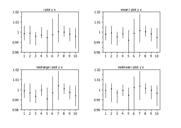
multiplot 2 2
i plot y x
mean i plot y x
midrange i plot y x
midmean i plot y x
end of multiplot
    



.
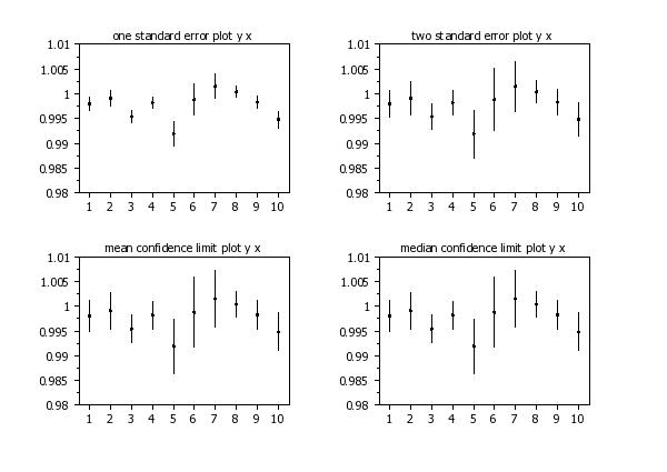
multiplot 2 2
one standard error plot y x
two standard error plot y x
mean confidence limit plot y x
median confidence limit plot y x
end of multiplot
.
    



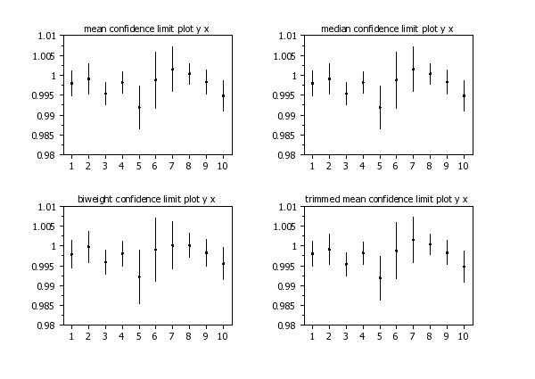
multiplot 2 2
mean confidence limit plot y x
median confidence limit plot y x
biweight confidence limit plot y x
trimmed mean confidence limit plot y x
end of multiplot
    

 
. Step 1:   Read the data
.
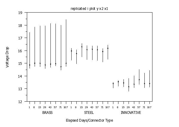
.           y = voltage drop
.           x1  = elapsed days (1, 8, 15, 29, 43, 57, 71, 107)
.           x2  = type of connector
.                 1 = brass
.                 2 = steel
.                 3 = innovative
skip 25
read clark0.dat  y days x2
let days = 8 subset days = 9
let days = 15 subset days = 16
let days = 29 subset days = 30
let days = 43 subset days = 44
let days = 57 subset days = 58
let days = 71 subset days = 72
let days = 107 subset days = 108
let x1 = coded days
let nx1 = unique x1
let nx2 = unique x2
let ntot = nx1*nx2
.
. Step 2:   I Plot with standard replication option
.
title case asis
title offset 2
label case asis
character case asis
line i plot
character blank circle blank blank blank
character fill off on
character hw 0.5 0.375 all
.
y1label Voltage Drop
x3label Elapsed Days/Connector Type
xlimits 1 ntot
major xtic mark number ntot
minor xtic mark number 0
x1tic mark offset 0.5 0.5
x1tic mark label format alpha
x1tic mark label content 1 8 15 29 43 57 71 107 1 8 15 29 43 57 71 107 ...
      1 8 15 29 43 57 71 107 
x1tic mark label size 1.6
title automatic
replicated i plot y x2 x1
.
justification center
let xcoor = (nx1/2) + 0.5
let ycoor = 10
moveds xcoor ycoor
text Brass
let xcoor = xcoor + nx1
moveds xcoor ycoor
text Steel
let xcoor = xcoor + nx1
moveds xcoor ycoor
text Innovative
    



.
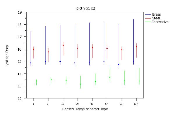
. Step 3:   I Plot with alternative replication option
.
line i plot bl bl bl so so bl bl bl so so bl bl bl so so
character bl circ bl bl bl bl circ bl bl bl bl circ bl bl bl
character fill on all
character hw 0.5 0.375 all
character color blue blue blue blue blue red red red red red ...
                green green green green green
line color blue blue blue blue blue red red red red red ...
           green green green green green
.
x1label Elapsed Days/Connector Type
x3label
xlimits 1 nx1
major xtic mark number nx1
minor xtic mark number 0
x1tic mark offset 0.5 0.5
x1tic mark label format alpha
x1tic mark label content 1 8 15 29 43 57 71 107
title automatic
i plot y x1 x2
    

 
. Step 1:   Read the data
.
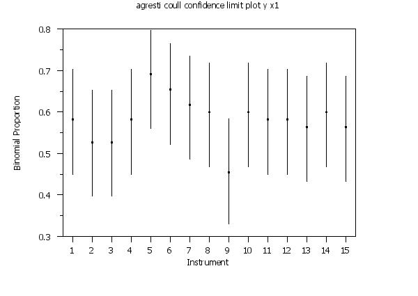
.           x1  = instrument
.           x2  = source
.           y1  = expected alarm
.           y2  = observed alarm
.           y   = 1 if y1 and y2 agree, 0 otherwise
skip 25
read alarm.dat  x1 x2 y1 y2
skip 0
let n = size y1
let y = 0 for i = 1 1 n
let y = 1 subset y1 = 0 subset y2 = 0
let y = 1 subset y1 = 1 subset y2 = 1
let ninst = unique x1
let nsrc  = unique x2
.
.
. Step 2:   I Plot with standard replication option
.
line i plot
character blank circle blank blank blank
character fill off on
character hw 0.5 0.375 all
.
label case asis
title case asis
y1label Binomial Proportion
x1label Instrument
xlimits 1 ninst
major xtic mark number ninst
minor xtic mark number 0
x1tic mark offset 0.5 0.5
title automatic
agresti coull confidence limit plot y x1
.
difference of proportion confidence limit plot y1 y2 x1