BOX PLOT

BOX PLOT

Graphics Command

Generates a box plot.

A box plot is a graphical data analysis technique for determining if differences exist between the various levels of a 1-factor model. It is a graphical alternative to 1-factor ANOVA. It consist of:

Vertical axis	=	response variable;
Horizontal axis	=	level identification.

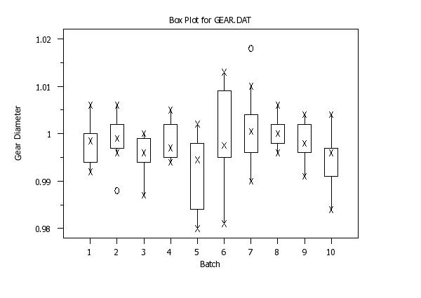
The bottom x is the data minimum; the bottom of the box is the estimated 25% point; the middle x in the box is the data median; the top of the box is the estimated 75% point; the top x is the data maximum. The box plot has 24 components (characters and lines) which may be individually controlled. For the box plot to appear as it should, the BOX PLOT command is usually preceded by two commands--

CHARACTERS BOX PLOT
LINES BOX PLOT


which will automatically define proper values for the 24 components of the box plot. After the box plot is formed, the analyst should redefine plot characters and lines via the usual CHARACTERS and LINES commands.

BOX PLOT <y>             <SUBSET/EXCEPT/FOR qualification>
where <y> is the response (= dependent) variable;
and where the <SUBSET/EXCEPT/FOR qualification> is optional.

This syntax generates a single box. Note that <y> can also be a matrix argument. If <y> is a matrix, a single box is drawn for all the values in the matrix.

BOX PLOT <y> <x>             <SUBSET/EXCEPT/FOR qualification>
where <y> is the response (= dependent) variable;
            <x> is an independent variable;
and where the <SUBSET/EXCEPT/FOR qualification> is optional.

MULTIPLE BOX PLOT <y1> ... <yk>
                        <SUBSET/EXCEPT/FOR qualification>
where <y1> ... <yk> is a list of response (= dependent) variables;
and where the <SUBSET/EXCEPT/FOR qualification> is optional.

Note that response variables can also be matrices. If a matrix name is encountered, a box will be drawn for all the values in the matrix.

REPLICATED BOX PLOT <y> <x1> ... <xk>
                        <SUBSET/EXCEPT/FOR qualification>
where <y> is the response (= dependent) variable;
            <x1> ... <xk> is a list of 1 to 6 group-id variables;
and where the <SUBSET/EXCEPT/FOR qualification> is optional.

The group-id variables are cross-tabulated and a box is drawn for each distinct combination of values for the group-id variables. These are sometimes referred to as nested box plots.

For the REPLICATED case, you can control the spacing between groups. Internally, Dataplot uses the CODE CROSS TABULATE command to generate a single combined group-id variable. Enter HELP CODE CROSS TABULATE for details on the ordering of the cross-tabulation and on how to control the spacing (the SET commands used by CODE CROSS TABULATE are supported for the BOX PLOT command).

BOX PLOT Y X
BOX PLOT Y X1
MULTIPLE BOX PLOT Y1 TO Y10
REPLICATED BOX PLOT Y X1 TO X4

Outliers can be identified by entering the FENCES ON command. If the inter-quartile range (i.e., the difference between the 25% point and the 75% point) is IQ, then values that are between 1.5 and 3.0 times the IQ above (or below) the 75% point (or the 25%) point are drawn as circles and points that are more than 3.0 times the IQ above (or below) the 75% point (or the 25%) are drawn as large circles.

The width of the box is proportional to the number of data points in that box.

If you want to generate fixed width box plots, enter the command

SET BOX PLOT WIDTH FIXED

To restore variable width box plots, enter the command

SET BOX PLOT WIDTH VARIABLE

An alternate form of the box plot can be generated by entering the commands CHARACTERS TUFTE BOX PLOT and LINES TUFTE BOX PLOT. You can also define your own plot symbols with the standard CHARACTER and LINE commands (e.g., you may prefer to use a dash (-) rather than the default X.

The TO syntax is supported for the BOX PLOT command. It is most useful for the MULTIPLE and REPLICATED versions of the commands.

If you use MEAN BOX PLOT rather than BOX PLOT, Dataplot will generate the plot based on the mean and standard deviations rather than the median and lower and upper hinges.

The commands LINES BOX PLOT and CHARACTER BOX PLOT actually define 24 components:

1	-	character at maximum point (if FENCES OFF) character at upper adjacent point (if FENCES ON)
2	-	character at top of the box (upper hinge)
3	-	character in the box but towards the top of the box (such as upper confidence level for mean, if any)
4	-	define the character for the median (or mean)
5	-	character in the box but towards the bottom of the box (such as lower confidence level for mean, if any)
6	-	character at bottom of the box (lower hinge)
7	-	character at minimum point (if FENCES OFF) character at lower adjacent point (if FENCES ON)
8	-	vertical line from maximum value to the top of the box (if FENCES (OFF) vertical line from upper adjacent value to the top of the box (if FENCES (ON)
9	-	vertical line from the top of the box to the point in the box towards the top of the box (such as upper confidence level for mean, if any)
10	-	vertical line from the point in the box toward the top (such as the upper confidence limit point) to the median (or mean)
11	-	vertical line from the median (or mean) to the point in the box toward the bottom (such as the lower confidence limit point)
12	-	vertical line from the point in the box toward the bottom (such as the lower confidence limit point) to the bottom of the box
13	-	vertical line from minimum value to the bottom of the box (if FENCES (OFF) vertical line from lower adjacent value to the bottom of the box (if FENCES (ON)
14	-	vertical line constituting the left side of the box
15	-	vertical line constituting the right side of the box
16	-	horizontal line at the top of the box
17	-	horizontal line at the bottom of the box
18	-	horizontal line running through the median (or mean)
19	-	horizontal line running through the lower confidence limit
20	-	horizontal line running through the upper confidence limit
21	-	characters for the upper far out values
22	-	characters for the upper near out values
23	-	characters for the lower near out values
24	-	characters for the lower far out values

The 2016/06 version of Dataplot no longer treats a single point for the response variable or all values in the response variable as being an error. Box plots are not typically drawn for a small number of points. However, when automating the analysis for a large data set, it can be more desirable to have these cases treated as degenerate cases rather than as errors.

To have a horizontal bars drawn at the 1%, 5%, 10%, 90%, 95%, and 99% points of the distribution, enter
SET BOX PLOT EXTREME PERCENTILES ON

This option may be useful for large data sets.

If the FENCES switch is OFF, then the CHARACTER and LINE settings for traces 21 through 26 will be used to draw these percentiles. If the FENCES switch is ON, then the CHARACTER and LINE settings for traces 25 through 30 will be used to draw these percentiles. Currently, the LINES BOX PLOT and CHARACTER BOX PLOT commands do not set these. You can use something like the following to set these switches.

LET INDX = DATA 21 22 23 24 25 26
LET PLOT CHARACTER INDX = BLANK
LET PLOT LINE INDX = SOLID

If you use the MULTIPLE syntax as in the following example
MULTIPLE BOX PLOT Y1 Y2 Y3 Y4 Y5

Dataplot will internally create a stacked Y X set of data. This means that Dataplot's limit on the maximum number of rows applies to the combined number of rows in the response variables. Dataplot was modified so that if there are four or fewer response variables, then Dataplot will not stack the data to generate the box plot. Although this has no effect on the appearance of the plot, it can be useful when generating box plots for large data sets in that it may avoid exceeding Dataplot's limit on the maximum number of rows.

The FENCES ON command is used to help identify outliers. One criticism of the box plot is that the method used identifies too many potential outliers for skewed data.

Walker proposed the following alternative for the fences

\[ f_{L} = q_1 - 1.5 \mbox{ IQR } \frac{\mbox{SIQR}_{L}} {\mbox{SIQR}_{U}} \]
\[ f_{U} = q_1 - 1.5 \mbox{ IQR } \frac{\mbox{SIQR}_{U}} {\mbox{SIQR}_{L}} \]

where

\( q_1 \)	=	the lower quartile
\( q_3 \)	=	the upper quartile
IQR	=	the interquartile range
	=	\( q_3 - q_1 \)
\( \mbox{SIQR}_L \)	=	the lower semi-interquartile range
	=	\( q_2 - q_1 \)
\( \mbox{SIQR}_U \)	=	the upper semi-interquartile range
	=	\( q_3 - q_2 \)
\( q_2 \)	=	the median

This formulation is based on the Galton (or Bowley) formula for skewness

\( B_c \)	=	\( \frac{q_2 + q_1 - 2 q_2} {q_3 - q_1} \)
	=	\( \frac{\mbox{SIQR}_U - \mbox{SIQR}_L} {\mbox{IQR}} \)
	=	\( \frac{\mbox{SIQR}_U - \mbox{SIQR}_L} {\mbox{SIQR}_U + \mbox{SIQR}_L} \)

For a more complete explanation of this method, see the Walker paper.

Kimber had earlier proposed

\[ f_{L} = q_1 - 1.5 (2(q_2 - q_1)) \]
\[ f_{U} = q_3 + 1.5 (2(q_3 - q_2)) \]

For skewed data, the Kimber method tends to be intermediate between the default method and the Walker method in the number of potential outliers it identifies. For symmetric data, the Kimber and Walker methods are essentially equivalent to the default method. However, for skewed data, the Kimber and Walker methods will identify fewer potential outliers than the default method.

The above formulas are for the "inner fences" boundary. For the "outer fences" boundary, replace 1.5 with 3.0.

To use the Walker method, enter the command

SET BOXPLOT FENCE SKEWNESS WALKER

To use the Kimber method, enter the command

SET BOXPLOT FENCE SKEWNESS KIMBER

To reset the default method, enter

SET BOXPLOT FENCE SKEWNESS OFF

Note that using the Walker or Kimber methods is recommended when you are specifically interested in identifying outliers. For exploratory purposes, it may be preferrable to use the default method (i.e., showing the skewness may be desirable).

None

The word REPLICATED is optional in the REPLICATED BOX PLOT syntax.
SET BOXPLOT FENCE SKEWNESS OFF and SET BOXPLOT FENCE SKEWNESS BOWLEY are synonyms for SET BOXPLOT FENCE SKEWNESS WALKER.

CHARACTERS	= Sets the types for plot characters.
LINES	= Sets the types for plot lines.
I PLOT	= Generates an I plot.
ANOVA	= Carries out an ANOVA.
MEDIAN POLISH	= Carries out a median polish.
CONTROL CHART	= Generates a control chart.
PLOT	= Generates a data or function plot.

Tukey (1977), "Exploratory Data Analysis," Addison-Wesley.

Walker, Dovedo, Chakraborti and Hilton (2019), "An Improved Boxplot for Univariate Data", The American Statistician, Vol. 72, No. 4, pp. 348-353.

Kimber (1990), "Exploratory Data Analysis for Possibly Censored Data from Skewed Distribution", Applied Statistics, Vol. 39, pp. 21-30.

Exploratory Data Analysis, Comparing Distributions

Pre-1987
2002/3: Support for fixed width box plot
2010/6: Support for TO syntax and matrix arguments
2010/6: Support for MULTIPLE and REPLICATED options
2016/06: Sample size of one or all response values having the same value no longer treated as an error
2016/06: Support for the SET BOX PLOT EXTREME PERCENTILES
2016/06: For MULTIPLE option, four or fewer response variables not stacked internally
2019/08: Support for the SET BOXPLOT FENCE SKEWNESS command

 
SKIP 25
READ GEAR.DAT Y X
.
TITLE CASE ASIS
TITLE OFFSET 2
LABEL CASE ASIS
TITLE Box Plot for GEAR.DAT
Y1LABEL Gear Diameter
X1LABEL Batch
.
TIC MARK OFFSET UNITS DATA
XLIMITS 1 10
MAJOR XTIC MARK NUMBER 10
MINOR XTIC MARK NUMBER 0
XTIC MARK OFFSET 1  1
YTIC MARK OFFSET 0.002 0.002
.
LINES BOX PLOT
CHARACTER BOX PLOT
CHARACTER FONT SIMPLEX ALL
FENCES ON
BOX PLOT Y X
    

 
dimension 40 columns
skip 25
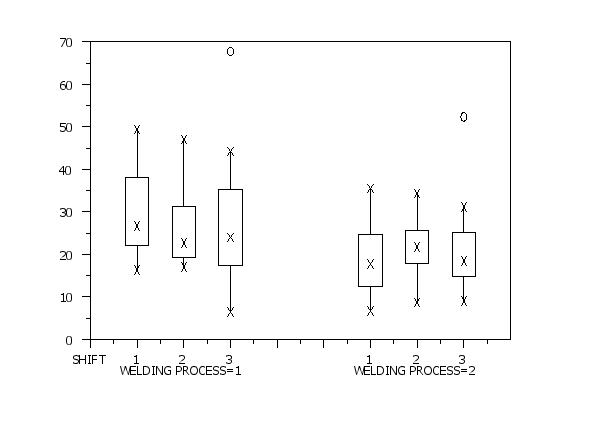
read sheesley.dat y x1 to x5
let x1d = distinct x1
let x2d = distinct x2
.
SET CODE CROSS TABULATE GROUP SIZE ONE 5
xlimits 0 8
xtic mark offset 0 1
major xtic mark number 9
x1tic mark label format alpha
x1tic mark label content Shift 1 2cr()Weldingsp()Process=1 3 sp() sp() ...
      1 2cr()Weldingsp()Process=2 3
.
character box plot
character font simplex all
lines box plot
fences on
.
box plot y x1 x2
.
    



 
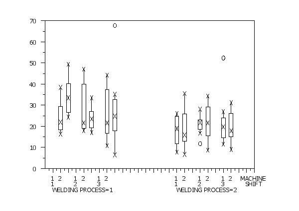
SET CODE CROSS TABULATE GROUP SIZE ONE 5
SET CODE CROSS TABULATE GROUP SIZE TWO 3
xlimits 0 26
xtic mark offset 1 0
major xtic mark number 27
set string space ignore
let string s1 = 1cr()1
let string s2 = 2
let string s3 = sp()
let string s4 = 1cr()2
let string s5 = 2cr()sp()cr()Weldingsp()Process=1
let string s6 = sp()
let string s7 = 1cr()3
let string s8 = 2
let string s9 = sp()
let string s10 = sp()
let string s11 = sp()
let string s12 = sp()
let string s13 = sp()
let string s14 = sp()
let string s15 = sp()
let string s16 = sp()
let string s17 = 1cr()1
let string s18 = 2
let string s19 = sp()
let string s20 = 1cr()2
let string s21 = 2cr()sp()cr()Weldingsp()Process=2
let string s22 = sp()
let string s23 = 1cr()3
let string s24 = 2
let string s25 = sp()
let string s26 = sp()
let string s27 = Machinecr()Shift
let igx = group label s1 to s27
.
x1tic mark label format group label
x1tic mark label content igx
box plot y x1 x2 x3
    



 
.
reset data
skip 25
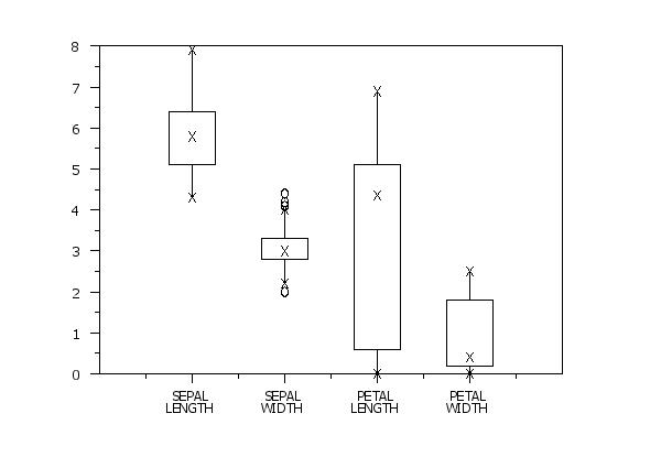
read iris.dat y1 y2 y3 y4 species
let m = create matrix y1 y2 y3 y4
.
xlimits 1 4
xtic mark offset 1 1
major xtic mark number 4
x1tic mark label format alpha
x1tic mark label content Sepalcr()Length Sepalcr()Width ...
      Petalcr()Length Petalcr()Width
multiple box plot m1 m2 m3 m4
    



 
.
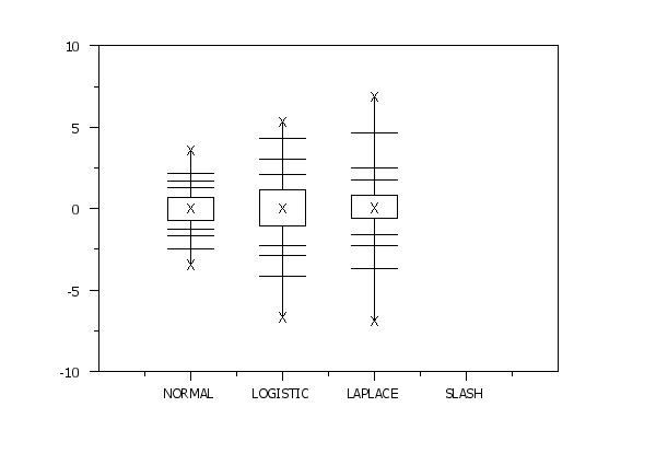
reset data
let y1 = norm rand numb for i = 1 1 1000
let y2 = logistic rand numb for i = 1 1 1000
let y3 = double exponential rand numb for i = 1 1 1000
let y4 = slash rand numb for i = 1 1 1000
.
xlimits 1 4
xtic mark offset 1 1
major xtic mark number 4
x1tic mark label format alpha
x1tic mark label content Normal Logistic Laplace Slash
      Petalcr()Length Petalcr()Width
set box plot extreme percentiles on
.
.  Reset character/line settings above 20
.
fences off
loop for k = 21 1 26
    let plot character ^k = blank
    let plot line      ^k = solid
end of loop
.
multiple box plot y1 y2 y3
    

 
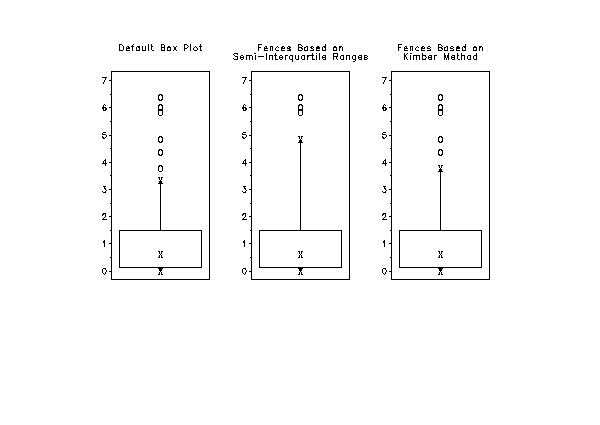
. Step 1:   Create data (skewed)
.
let nu = 1
let y = chisquare random numbers for i = 1 1 100
.
. Step 2:   Define plot control
.
character box plot
line box plot
fences on
title case asis
x1tic marks off
x1tic mark labels off
tic mark offset units screen
y1tic mark offset 3 3
.
. Step 3:   Generate the box plots
.
multiplot 1 3
multiplot scale factor 1 3
title Default Box Plot
box plot y
set box plot fence skewness galton
title Fences Based oncr()Semi-Interquartile Ranges
box plot y
set box plot fence skewness kimber
title Fences Based oncr()Kimber Method
box plot y
.
end of multiplot