|
|
EMPIRICAL QUANTILE PLOTName:
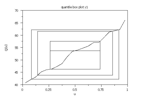
\( \frac{2j - 1}{2n} \le u \le \frac{2j + 1}{2n} \) This will be computed for a specified number of equi-spaced points between the lower and upper limits. Dataplot will use the minimum of 1,000 points and the number of points in the sample. This plot is essentially the inverse of the empirical CDF plot. The empirical quantile plot can be enhanced with an overlaid quantile box plot (see Syntax 4). The QUANTILE BOX PLOT command will first generate the empirical quantile plot and then it will overlay the quantile box plot. The quantile box plot draws the following rectangles:
The quantile box plot can help in assesing the symmetry, tail behavior, and the presence of outliers of the underlying distribution of the data. These plots are suggested as exploratory data analysis techniques in the MIL-HANDBK-17 (2002 edition). They were originally suggested by Parzen (see References below).
<SUBSET/EXCEPT/FOR qualification> where <y> is a response variable; and where the <SUBSET/EXCEPT/FOR qualification> is optional.
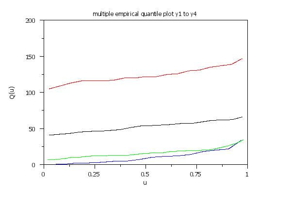
<SUBSET/EXCEPT/FOR qualification> where <y1> ... <yk> is a list of 1 to 30 response variables; and where the <SUBSET/EXCEPT/FOR qualification> is optional. This syntax generates an empirical quantile plot for each listed response variable. These response variables can be matrices. The TO syntax is supported for this case.
<SUBSET/EXCEPT/FOR qualification> where <y> is a response variable; <x1> is the first (required) group-id variables; <x2> is the second (optional) group-id variables; and where the <SUBSET/EXCEPT/FOR qualification> is optional. This syntax peforms a cross-tabulation of <x1> and <x2> and generates the quantile function plot for each unique combination of cross-tabulated values. For example, if X1 has 3 levels and X2 has 2 levels, there will be a total of 6 plots generated.
where <y> is a response variable containing failure times; and where the <SUBSET/EXCEPT/FOR qualification> is optional. The MULTIPLE and REPLICATED options are not supported for this syntax.
EMPIRICAL QUANTILE PLOT Y1 SUBSET TAG > 1 MULTIPLE EMPIRICAL QUANTILE PLOT Y1 Y2 Y3 Y4 Y5 MULTIPLE EMPIRICAL QUANTILE PLOT Y1 TO Y5 REPLICATED EMPIRICAL QUANTILE PLOT Y X
Parzen (1983), "Informative Quantile Functions and Identification of Probability Distribution Types", Technical Report No. A-26, Texas A&M University.
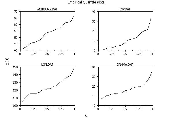
. Step 1: Read the data . skip 25 read weibbury.dat y1 read exp.dat y2 read lgn.dat y3 read gamma.dat y4 . . Step 2: Define some default plot control features . title offset 2 title case asis case asis label case asis line color blue red multiplot scale factor 2 multiplot corner coordinates 5 5 95 95 . . Step 3: Generate the empirical quantile plot . multiplot 2 2 . title WEIBBURY.DAT empirical quantile plot y1 . title EXP.DAT empirical quantile plot y2 . title LGN.DAT empirical quantile plot y3 . title GAMMA.DAT empirical quantile plot y4 . end of multiplot . justification center move 50 97 text Empirical Quantile Plots move 50 5 text u direction vertical move 5 50 text Q(u) 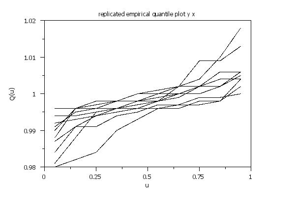
Date created: 06/29/2017 |
Last updated: 12/04/2023 Please email comments on this WWW page to [email protected]. | |||||||||||||||||||||||||