AVERAGE SHIFTED HISTOGRAM

AVERAGE SHIFTED HISTOGRAM

Graphics Command

Generates an average shifted histogram.

In addition to providing a convenient summary of a univariate set of data, the histogram can also be thought of as a simple kernel density estimator.

David Scott has proposed the average shifted histogram (see chapter 5 of the "Multivariate Density Estimation: Theory and Practice, and Visualization" listed in the Reference section below) as a kernel density estimator that maintains the computational simplicity of the histogram while providing performance comparable to the more computationally intensive kernel density plot (enter HELP KERNEL DENSITY PLOT for details on the kernel density plot).

The basic algorithm for the average shifted histogram is:

1. Choose a class width of h (in Dataplot, you can select this class width with either the CLASS WIDTH or the SET HISTOGRAM CLASS WIDTH command, otherwise a default class width of 0.3 times the sample standard deviation will be used).

2. Choose m where we construct a collection of m histograms, each with a class width of h, but with start points t₀ = 0, h/m, 2h/m, ... , (m-1)h/m.

   In Dataplot, the value of m is set by entering the command

   LET M = <value>

   before entering the AVERAGE SHIFTED HISTOGRAM command.

   If the number of points is less than or equal to 100, the default value is 4. If the number of points is less than or equal to 1,000, the default value is 8. If the number of points is greater than 1,000, the default value is 16.

   Dataplot sets values of m < 1 to 1 and values of m > 64 to 64.

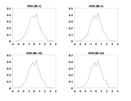
3. This results in a "smoothed" histogram with a bin width of delta=h/m. Higher values of m result in a smoother estimate. Values of m are typically in the range 4 to 32.

This is the algorithm given on page 117 of Scott. This effectively gives an isosceles triangle weighting function. Scott gives a generalization of the ASH algorithm that gives a biweight weighting function. This is the ASH1 algorithm on page 118. This will generate a smoother curve with less local noise than the triangular weighting.

To use this biweight weighting function, enter the command

SET AVERAGE SHIFTED HISTOGRAM WEIGHT BIWEIGHT

To restore the default triangular weighting, enter

SET AVERAGE SHIFTED HISTOGRAM WEIGHT TRIANGULAR

AVERAGE SHIFTED HISTOGRAM <x>
                        <SUBSET/EXCEPT/FOR qualification>
where <x> is the variable of raw data values;
and where the <SUBSET/EXCEPT/FOR qualification> is optional.

AVERAGE SHIFTED HISTOGRAM TEMP
AVERAGE SHIFTED HISTOGRAM Y SUBSET TAG = 2
AVERAGE SHIFTED HISTOGRAM Y FOR I = 1 1 800

Dataplot implements average shifted histograms using the algorithms BIN1 and ASH1 given on pages 117-118 of the Scott book.

The average shifted histogram can be adapted to higher dimensional data. It is this multivariate case where the computational simplicity (relative to the kernel density plot) is particularly attractive. At this time, we have not implemented the multivariate case. We do plan to implement it in a future release.

The AVERAGE SHIFTED HISTOGRAM command generates an estimate of the underlying density function. You can convert this to an estimate of the cumulative distribution function by integrating the density estimate. The following shows an example of doing this in Dataplot.
LET Y = NORMAL RANDOM NUMBERS FOR I = 1 1 1000
AVERAGE SHIFTED HISTOGRAM Y
LET YPDF = YPLOT
LET XPDF = XPLOT
LET YCDF = CUMULATIVE INTEGRAL YPDF XPDF
TITLE ESTIMATE OF UNDERLYING CUMULATIVE DISTRIBUTION
PLOT YCDF XPDF


You can also obtain an estimate of the percent point function (inverse cdf) with the following additional commands:

LET YPPF = XCDF
LET XPPF = YCDF

None

ASH is a synonym for the AVERAGE SHIFTED HISTOGRAM command.

KERNEL DENSITY PLOT	= Generates a kernel density plot.
HISTOGRAM	= Generates a histogram.
FREQUENCY PLOT	= Generates a frequency plot.
CLASS WIDTH	= Set the class width for a histogram.
HISTOGRAM CLASS WIDTH	= Set the default class width algorithm for a histogram.

David Scott (1992), "Multivariate Density Estimation," John Wiley, (chapter 5 in particular).

B. W. Silverman (1986), "Density Estimation for Statistics and Data Analysis," Chapman & Hall.

Density Estimation

2004/9

 
LET Y = NORMAL RANDOM NUMBERS FOR I = 1 1 1000
TITLE OFFSET 2
MULTIPLOT CORNER COORDINATES 0 0 100 100
MULTIPLOT SCALE FACTOR 2
MULTIPLOT 2 2
LET M = 1
TITLE ASH (M=1)
AVERAGE SHIFTED HISTOGRAM Y
LET M = 4
TITLE ASH (M=4)
AVERAGE SHIFTED HISTOGRAM Y
LET M = 16
TITLE ASH (M=16)
AVERAGE SHIFTED HISTOGRAM Y
LET M = 32
TITLE ASH (M=32)
AVERAGE SHIFTED HISTOGRAM Y
END OF MULTIPLOT