KERNEL DENSITY PLOT

KERNEL DENSITY PLOT

Graphics Command

Generates a kernel density plot.

The kernel density estimate, f(n), of a set of n points from a density f is defined as:
\( f_n(x) = \frac{\sum_{j=1}^{n}{K\{\frac{(x - X_j)}{h}\}}} {nh} \)

where K is the kernel function and h is the smoothing parameter or window width.

Currently, Dataplot uses a Gaussian kernel function. This downweights points smoothly as the distance from x increases. The width parameter can be set by the user (see Note: below), although Dataplot will provide a default width that should produce reasonable results for most data sets.

A kernel density plot can be considered a refinement of a histogram or frequency plot.

KERNEL DENSITY PLOT <y>             <SUBSET/EXCEPT/FOR qualification>
where <y> is the variable of raw data values;
and where the <SUBSET/EXCEPT/FOR qualification> is optional.

Note that <y> can be either a variable or a matrix. If <y> is a matrix, a kernel density plot will be generated for all values in the matrix.

MULTIPLE KERNEL DENSITY PLOT <y1> ... <yk>
                                                <SUBSET/EXCEPT/FOR qualification>
where <y1> ... <yk> is a list of response variables;
and where the <SUBSET/EXCEPT/FOR qualification> is optional.

This syntax will overlay multiple kernel density plots on the same plot.

Note that the response variables (<y1> ... <yk> can be either variables or matrices (or a mix of variables and matrices). For matrices, a kernel density plot will be generated for all values in the matrix.

REPLICATED KERNEL DENSITY PLOT <y> <x1>
                                                <SUBSET/EXCEPT/FOR qualification>
where <y> is the variable of raw data values;
                        <x1> is a group-id variable;
and where the <SUBSET/EXCEPT/FOR qualification> is optional.

This syntax will generate a kernel density plot for each distinct value in the group-id variable. The kernel density plots will be generated on the same page.

REPLICATED KERNEL DENSITY PLOT <y> <x1> <x2>
                                                <SUBSET/EXCEPT/FOR qualification>
where <y> is the variable of raw data values;
                        <x1> is the first group-id variable;
                        <x2> is the second group-id variable;
and where the <SUBSET/EXCEPT/FOR qualification> is optional.

This syntax will cross tabulate the group-id variables and generate a kernel density plot for each unique combination of values for the <x1> and <x2> group-id variables. The kernel density plots will be generated on the same page.

KERNEL DENSITY PLOT TEMP
KERNEL DENSITY PLOT Y SUBSET TAG = 2
KERNEL DENSITY PLOT Y FOR I = 1 1 800
MULTIPLE KERNEL DENSITY PLOT Y1 Y2 Y3
REPLICATED KERNEL DENSITY PLOT Y X1 X2

Dataplot computes the kernel density estimate using Algorithm 176 from Applied Statistics (see Reference below). This code was contributed by B. W. Silverman.

This algorithm is based on the Fast Fourier Transform (FFT). The use of the FFT results in much greater computational efficiency. The article that accompanies this algorithm provides the details of how the FFT is used and provides timing estimates of this implemenation relative to an algorithm based on the definition of the kernel function.

By default, the density curve is generated with 256 points. Note that this is the number of points on the density curve, not the number of points in the raw data.

You can set the number of points for the density curve using the following command:

KERNEL DENSITY POINTS <value>

where <value> defines the number of points.

Following the recommendation of Silverman (1986), DATAPLOT uses a default width of
\( 0.9 \min(s,\mbox{IQ}/1.34) n^{-1/5} \)

where s is the sample standard deviation and IQ is the sample interquartile range. Silverman provides justification for this choice. Basically, it should perform reasonably for a wide variety of distributions. Note that the optimal width depends on the underlying function, which is what we are trying to estimate.

If the underlying data is in fact normally distributed, then Silverman (1986) shows that the optimal width is

\( 1.06 s n^{-1/5} \)

where n is the number of points in the raw data and s is the sample standard deviation of the raw data.

It may be worthwhile to generate the density curve using several different values for the width. Silverman also recommends trying to transform skewed data sets to be symmetric.

The width can be set with the following command:

KERNEL DENSITY WIDTH <value>

Dataplot will not generate the density curve unless the input data set contains at least 20 data points. In fact, the sample size should be larger than this for density plots to be an appropriate mehtod.

The KERNEL DENSITY PLOT estimates the underlying probability density function. However, it can also be used to estimate the cumulative distribution function (cdf) or the percent point function (ppf). To estimate the cdf, the cumulative integral of the kernel density plot is computed. The ppf is inverse of the cdf, so the role of the x and y values from the estimated cdf are switched to obtain an estimate of the ppf function.

To plot the estimated cdf, enter

SET KERNEL DENSITY PROBABILITY FUNCTION CDF

To plot the estimated ppf, enter

SET KERNEL DENSITY PROBABILITY FUNCTION PPF

To reset the plotting of the pdf, enter

SET KERNEL DENSITY PROBABILITY FUNCTION PDF

Given that we can estimate the ppf function, we can use this to generate random numbers based on the kernel density plot. If you would like to generate random numbers, enter the command

SET KERNEL DENSITY RANDOM NUMBERS <value>

where <value> is a number between 1 and the maximum number of rows. If <value> is set to 0 or a negative number, no random numbers are generated.

Specifically, the following procedure is used:

1. Generate uniform random numbers (the uniform random numbers correspond to x-axis values on the ppf version of the kernel density plot).

2. From the ppf version of the kernel density plot, determine the y-axis value on the kernel density curve that corresponds to the x-axis value. Cubic spline interpolation is used to estimate the y-axis value. That is, at the points defined by the uniform random numbers, we find interpolated values based on the (x,y) coordinates of the kernel density curve.

3. The random numbers are written to the file dpst1f.dat using an E15.7 format.

Dataplot computes the density curve from
(YMINIMUM - 3*H, YMAXIMUM + 3*H)

where YMINIMUM and YMAXIMUM are the minimum and maximum values of the raw data and H is the window width.

The KERNEL DENSITY PLOT supports the TO syntax for the list of variable names. This is most useful for the MULTIPLE case.

The default window width is \( 1.06 s n^{-1/5} \) where n is the number of points in the raw data and s is the sample standard deviation. The density trace is generated with 256 points.

The following are synonyms for the KERNEL DENSITY PLOT command.
KERNEL PLOT
DENSITY PLOT
DENSITY TRACE


The word MULTIPLE is optional for the MULTIPLE KERNEL DENSITY PLOT command.

HISTOGRAM	= Generates a histogram.
FREQUENCY PLOT	= Generates a frequency plot.
KERNEL DENSITY WIDTH	= Sets the width factor, h, for the kernel density plot.
KERNEL DENSITY POINTS	= Sets the number of points generated for the kernel density plot.

B. W. Silverman (1982), "Kernel Density Estimation using the Fast Fourier Transform," Applied Statistics, Royal Statistical Society, Vol. 33.

B. W. Silverman (1986), "Density Estimation for Statistics and Data Analysis," Chapman & Hall.

David Scott (1992), "Multivariate Density Estimation," John Wiley.

Density Estimation

2001/08
2010/02: Support for the MULTIPLE and REPLICATION syntax
2010/02: Support for matrix arguments and the TO syntax
2018/07: Support for SET KERNEL DENSITY PROBABILITY FUNCTION
2018/07: Support for SET KERNEL DENSITY RANDOM NUMBERS

MULTIPLOT SCALE FACTOR 2
MULTIPLOT 2 2
MULTIPLOT CORNER COORDINATES 0 0 100 100
.
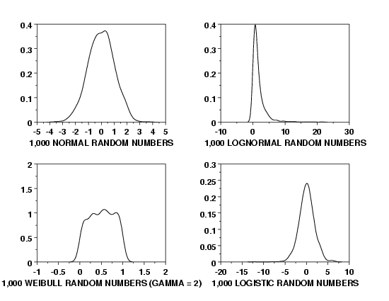
LET Y = NORMAL RANDOM NUMBERS FOR I = 1 1 1000
X3LABEL 1,000 NORMAL RANDOM NUMBERS
KERNEL DENSITY PLOT Y
.
LET Y = LOGNORMAL RANDOM NUMBERS FOR I = 1 1 1000
X3LABEL 1,000 LOGNORMAL RANDOM NUMBERS
KERNEL DENSITY PLOT Y
.
LET GAMMA = 2
LET Y = WEIBULL RANDOM NUMBERS FOR I = 1 1 1000
X3LABEL 1,000 WEIBULL RANDOM NUMBERS (GAMMA = 2)
KERNEL DENSITY PLOT Y
.
LET Y = LOGISTIC RANDOM NUMBERS FOR I = 1 1 1000
X3LABEL 1,000 LOGISTIC RANDOM NUMBERS
KERNEL DENSITY PLOT Y
END OF MULTIPLOT
    

. Step 1:   Read the data
.
skip 25
read zarr13.dat y
skip 0
.
. Step 2:   Plot control features
.
multiplot corner coordinates 5 5 95 95
multiplot scale factor 2
title offset 2
title case asis
label case asis
case asis
.
. Step 3:   Generate the kernel density plot
.
multiplot 2 2
.
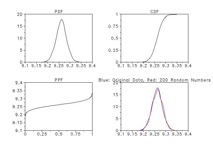
title PDF
kernel density plot y
.
title CDF
set kernel density probability function cdf
kernel density plot y
.
title PPF
set kernel density probability function ppf
set kernel density random numbers 200
kernel density plot y
.
read dpst1f.dat yrand
line color blue red
title Blue: Original Data, Red: 200 Random Numbers
set kernel density probability function pdf
multiple kernel density plot y yrand
.
end of multiplot