5. Process Improvement
5.5. Advanced topics
5.5.5. How do you optimize a process?
5.5.5.2. Multiple response case

5.5.5.2.2.

Multiple response: The desirability approach

The desirability approach is a popular method that assigns a "score" to a set of responses and chooses factor settings that maximize that score
 
 
 
 
 
 
 
 
 
 
 
 
 
 
 
 
 
 
 
 
 
 
 
 
 
 
 
 
 
 
 
 
 
 
 
 
 
 
 
 
 
 
 

Desirability approach steps
 
 
 
 
 

An example using the desirability approach
 
 
 
 
 
 

 

The desirability function approach is one of the most widely used methods in industry for dealing with the optimization of multiple response processes. It is based on the idea that the "quality'' of a product or process that has multiple quality characteristics, with one of them outside of some "desired" limits, is completely unacceptable. The method finds operating conditions  that provide the "most desirable'' response values.

For each response , a desirability function  assigns numbers between 0 and 1 to the possible values of , with  representing a completely undesirable value of  and  representing a completely desirable or ideal response value. The individual desirabilities are then combined using the geometric mean, which gives the overall desirability D:

 where k denotes the number of responses. Notice that if any response i is completely undesirable  then the overall desirability is zero. In practice, fitted response models  are used in the method.

Depending on whether a particular response  is to be maximized, minimized, or assigned to a target value, different desirability functions  can be used. A useful class of desirability functions was proposed by Derringer and Suich (1980). Let  and  be the lower, upper, and target values desired for response i, where . If a response is of the "target is best'' kind, then its individual desirability function is

where the exponents s and t determine how strictly the target value is desired. For s = t =1, the desirability function increases linearly towards , for s<1, t<1, the function is convex, and for s>1, t>1, the function is concave (see the example below for an illustration).

If a response is to be maximized instead, the individual desirability is instead defined as

where in this case  is interpreted as a large enough value for the response. Finally, if we want to minimize a response, we could use

where  represents a small enough value for the response.

The desirability approach consists of the following steps:

1. Conduct experiments and fit response models for all k responses;
2. Define individual desirability functions for each response;
3. Maximize the overall desirability D with respect to the controllable factors.

Example:

Derringer and Suich (1980) present the following multiple response experiment arising in the development of a tire tread compound. The controllable factors are : , hydrated silica level, , silane coupling agent level, and , sulfur level. The four responses to be optimized and their desired ranges are:

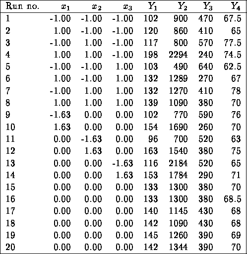
The first two responses are to be maximized, and the value s=1 was chosen for their desirability functions. The last two responses are "target is best'' with  and . The values s = t =1 were chosen in both cases. The following experiments were conducted according to a central composite design.

Using ordinary least squares and standard diagnostics, the fitted responses were:

 

(adj. );

(adj. );

(adj );

 

(adj. ).

Note that no interactions were significant for response 3, and that the fit for response 2 is quite poor.

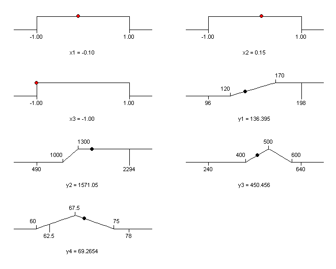
Optimization of D with respect to  was carried out using the Design Expert software. Figure 5.7 shows the individual desirability functions  for each of the four responses. The functions are linear since the values of s and t were selected equal to one. A dot indicates the best solution found by the Design Expert solver.

FIGURE 5.7  Desirability Functions and Optimal Solution for Example Problem

The best solution is  and results in


and . The overall desirability for this solution is 0.596. All responses are predicted to be within the desired limits.

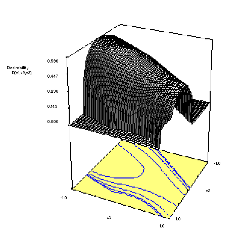
Figure 5.8 shows a 3D plot of the overall desirability function  for the  plane when  is fixed at -0.10. The function  is quite "flat'' in the vicinity of the optimal solution, indicating that small variations around  are not predicted to change the overall desirability drastically. However, it should be emphasized the importance of performing confirmatory runs at the estimated optimal operating conditions. This is particularly true in this example given the poor fit of the response models (e.g. ).

FIGURE 5.8  Overall Desirability Function for Example Problem