
|
6.
Process or Product Monitoring and Control
6.3. Univariate and Multivariate Control Charts 6.3.4. What are Multivariate Control Charts?
|
|||||||||||||||||||||||||||||||||||||||||||||||||||||||||||||||||||||||||||||||||||||||||||||||||||||||||||||||
| Multivariate EWMA Control Chart | |||||||||||||||||||||||||||||||||||||||||||||||||||||||||||||||||||||||||||||||||||||||||||||||||||||||||||||||
| Univariate EWMA model | The model for a univariate EWMA chart is given by: $$ Z_i = \lambda X_i + (1-\lambda)Z_{i-1}, \,\,\,\,\, i = 1, \, 2, \, \ldots, \, n \, , $$ where \(Z_i\) is the \(i\)th EWMA, \(X_i\) is the the \(i\)th observation, \(Z_0\) is the average from the historical data, and \(0 < \lambda \le 1\). | ||||||||||||||||||||||||||||||||||||||||||||||||||||||||||||||||||||||||||||||||||||||||||||||||||||||||||||||
| Multivariate EWMA model | In the multivariate case, one can extend this formula to $$ Z_i = \Lambda X_i + (1-\Lambda)Z_{i-1} \, , $$ where \(Z_i\) is the \(i\)th EWMA vector, \(X_i\) is the the \(i\)th observation vector \(i = 1, \, 2, \, \ldots, \, n\), \(Z_0\) is the vector of variable values from the historical data, \(\Lambda\) is the \(\mbox{diag}(\lambda_1, \, \lambda_2, \, \ldots, \, \lambda_p)\) which is a diagonal matrix with \(\lambda_1, \, \lambda_2, \, \ldots, \, \lambda_p\) on the main diagonal, and \(p\) is the number of variables; that is the number of elements in each vector. | ||||||||||||||||||||||||||||||||||||||||||||||||||||||||||||||||||||||||||||||||||||||||||||||||||||||||||||||
| Illustration of multivariate EWMA | The following illustration may clarify this. There are \(p\) variables and each variable contains \(n\) observations. The input data matrix looks like the following. $$ \begin{array}{cccc} X_{11} & X_{12} & \cdots & X_{1p} \\ X_{21} & X_{22} & \cdots & X_{2p} \\ \vdots & \vdots & \ddots & \vdots \\ & & & \\ X_{n1} & X_{n2} & \cdots & X_{np} \end{array} $$ The quantity to be plotted on the control chart is $$ T_i^2 = Z_i' \, \Sigma_{Z_i}^{-1} \, Z_i $$ | ||||||||||||||||||||||||||||||||||||||||||||||||||||||||||||||||||||||||||||||||||||||||||||||||||||||||||||||
| Simplification |
It has been shown (Lowry et al.,
1992) that the \( (k,l) \)th
element of the covariance matrix of the \(i\)th
EWMA, \(\Sigma_{Z_i}\),
is
$$ \Sigma_{Z_i}(k,l) = \lambda_k \lambda_l \,
\frac{\left[ 1-(1-\lambda_k)^i (1-\lambda_l)^i \right]}{(\lambda_k + \lambda_l - \lambda_k \lambda_l )} \,
\sigma_{k,l} \, , $$
where \(\sigma_{k,l}\)
is the \((k,l)\)th
element of \(\Sigma\),
the covariance matrix of the \(X\)'s.
If \(\lambda_1 = \lambda_2 = \cdots = \lambda_p = \lambda\), then the above expression simplifies to $$ \Sigma_{Z_i}(k,l) = \frac{\lambda}{2 - \lambda} \left[ 1-(1-\lambda)^{2i} \right] \Sigma \, , $$ where \(\Sigma\) is the covariance matrix of the input data. |
||||||||||||||||||||||||||||||||||||||||||||||||||||||||||||||||||||||||||||||||||||||||||||||||||||||||||||||
| Further simplification | There is a further simplification. When \(i\) becomes large, the covariance matrix may be expressed as: $$ \Sigma_{Z_i} = \frac{\lambda}{2 - \lambda} \Sigma \, . $$ The question is "What is large?". When we examine the formula with the \(2i\) in it, we observe that when \(2i\) becomes sufficiently large such that \((1-\lambda)^{2i}\) becomes almost zero, then we can use the simplified formula. | ||||||||||||||||||||||||||||||||||||||||||||||||||||||||||||||||||||||||||||||||||||||||||||||||||||||||||||||
| Table for selected values of \(\lambda\) and \(i\) |
The following table gives the values of \((1-\lambda)^{2i}\)
for selected values of \(\lambda\) and \(i\).
|
||||||||||||||||||||||||||||||||||||||||||||||||||||||||||||||||||||||||||||||||||||||||||||||||||||||||||||||
| Simplified formula not required | It should be pointed out that a well-meaning computer program does not have to adhere to the simplified formula, and potential inaccuracies for low values for \(\lambda\) and \(i\) can thus be avoided. | ||||||||||||||||||||||||||||||||||||||||||||||||||||||||||||||||||||||||||||||||||||||||||||||||||||||||||||||
| MEWMA computer output for the Lowry data |
Here is an example of the application of an MEWMA control chart. To
faciltate comparison with existing literature, we used data from
Lowry et al. The data were simulated from a bivariate normal
distribution with unit variances and a correlation coefficient
of 0.5. The value for \(\lambda = 0.10\)
and the values for \(T_i^2\)
were obtained by the equation
given above. The covariance of the MEWMA vectors was obtained
by using the non-simplified equation. That means that for each
MEWMA control statistic, the computer computed a covariance matrix,
where \(i = 1, \, 2, \, \ldots, \, 10\).
The results of the computer routine
are:
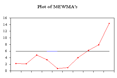
*****************************************************
*      Multi-Variate EWMA Control Chart             *
*****************************************************

DATA SERIES            MEWMA Vector          MEWMA
   1          2          1         2       STATISTIC
-1.190     0.590     -0.119     0.059        2.1886
 0.120     0.900     -0.095     0.143        2.0697
-1.690     0.400     -0.255     0.169        4.8365
 0.300     0.460     -0.199     0.198        3.4158
 0.890    -0.750     -0.090     0.103        0.7089
 0.820     0.980      0.001     0.191        0.9268
-0.300     2.280     -0.029     0.400        4.0018
 0.630     1.750      0.037     0.535        6.1657
 1.560     1.580      0.189     0.639        7.8554
 1.460     3.050      0.316     0.880       14.4158


VEC    XBAR      MSE      Lamda
 1     .260     1.200     0.100
 2    1.124     1.774     0.100
The UCL = 5.938 for \(\alpha = 0.05\). Smaller choices of \(\alpha\) are also used. |
||||||||||||||||||||||||||||||||||||||||||||||||||||||||||||||||||||||||||||||||||||||||||||||||||||||||||||||
| Sample MEWMA plot |
The following is the plot of the above MEWMA.
|
