1. Exploratory Data Analysis
1.3. EDA Techniques
1.3.3. Graphical Techniques: Alphabetic

1.3.3.33.

6-Plot

Purpose:
Graphical Model Validation

The 6-plot is a collection of 6 specific graphical techniques whose purpose is to assess the validity of a Y versus X fit. The fit can be a linear fit, a non-linear fit, a LOWESS (locally weighted least squares) fit, a spline fit, or any other fit utilizing a single independent variable.

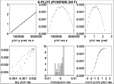
The 6 plots are:

1. Scatter plot of the response and predicted values versus the independent variable;
2. Scatter plot of the residuals versus the independent variable;
3. Scatter plot of the residuals versus the predicted values;
4. Lag plot of the residuals;
5. Histogram of the residuals;
6. Normal probability plot of the residuals.

Sample Plot

This 6-plot, which followed a linear fit, shows that the linear model is not adequate. It suggests that a quadratic model would be a better model.

Definition:
6 Component Plots

The 6-plot consists of the following:

1. Response and predicted values
   • Vertical axis: Response variable, predicted values
   • Horizontal axis: Independent variable
2. Residuals versus independent variable
   • Vertical axis: Residuals
   • Horizontal axis: Independent variable
3. Residuals versus predicted values
   • Vertical axis: Residuals
   • Horizontal axis: Predicted values
4. Lag plot of residuals
   • Vertical axis: RES(I)
   • Horizontal axis: RES(I-1)
5. Histogram of residuals
   • Vertical axis: Counts
   • Horizontal axis: Residual values
6. Normal probability plot of residuals
   • Vertical axis: Ordered residuals
   • Horizontal axis: Theoretical values from a normal N(0,1) distribution for ordered residuals

Questions

The 6-plot can be used to answer the following questions:

1. Are the residuals approximately normally distributed with a fixed location and scale?
2. Are there outliers?
3. Is the fit adequate?
4. Do the residuals suggest a better fit?

Importance:
Validating Model

A model involving a response variable and a single independent variable has the form:

\[ Y_{i} = f(X_{i}) + E_{i} \]

where Y is the response variable, X is the independent variable, f is the linear or non-linear fit function, and E is the random component. For a good model, the error component should behave like:

1. random drawings (i.e., independent);
2. from a fixed distribution;
3. with fixed location; and
4. with fixed variation.

In addition, for fitting models it is usually further assumed that the fixed distribution is normal and the fixed location is zero. For a good model the fixed variation should be as small as possible. A necessary component of fitting models is to verify these assumptions for the error component and to assess whether the variation for the error component is sufficiently small. The histogram, lag plot, and normal probability plot are used to verify the fixed distribution, location, and variation assumptions on the error component. The plot of the response variable and the predicted values versus the independent variable is used to assess whether the variation is sufficiently small. The plots of the residuals versus the independent variable and the predicted values is used to assess the independence assumption.

Assessing the validity and quality of the fit in terms of the above assumptions is an absolutely vital part of the model-fitting process. No fit should be considered complete without an adequate model validation step.

Related Techniques

Linear Least Squares
Non-Linear Least Squares
Scatter Plot
Run Sequence Plot
Lag Plot
Normal Probability Plot
Histogram

Case Study

The 6-plot is used in the Alaska pipeline data case study.

Software

It should be feasible to write a macro for the 6-plot in any general purpose statistical software program that supports the capability for multiple plots per page and supports the underlying plot techniques.