Skewness is a measure of symmetry, or more precisely, the lack of symmetry. A distribution, or data set, is symmetric if it looks the same to the left and right of the center point.

Kurtosis is a measure of whether the data are heavy-tailed or light-tailed relative to a normal distribution. That is, data sets with high kurtosis tend to have heavy tails, or outliers. Data sets with low kurtosis tend to have light tails, or lack of outliers. A uniform distribution would be the extreme case.

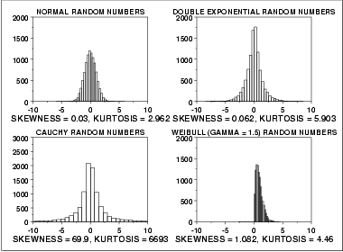
The histogram is an effective graphical technique for showing both the skewness and kurtosis of data set.

\[ g_{1} = \frac{\sum_{i=1}^{N}(Y_{i} - \bar{Y})^{3}/N} {s^{3}} \]

The above formula for skewness is referred to as the Fisher-Pearson coefficient of skewness. Many software programs actually compute the adjusted Fisher-Pearson coefficient of skewness

\[ G_{1} = \frac{\sqrt{N(N-1)}}{N-2} \frac{\sum_{i=1}^{N}(Y_{i} - \bar{Y})^{3}/N} {s^{3}} \]

The skewness for a normal distribution is zero, and any symmetric data should have a skewness near zero. Negative values for the skewness indicate data that are skewed left and positive values for the skewness indicate data that are skewed right. By skewed left, we mean that the left tail is long relative to the right tail. Similarly, skewed right means that the right tail is long relative to the left tail. If the data are multi-modal, then this may affect the sign of the skewness.

Some measurements have a lower bound and are skewed right. For example, in reliability studies, failure times cannot be negative.

It should be noted that there are alternative definitions of skewness in the literature. For example, the Galton skewness (also known as Bowley's skewness) is defined as

\[ \mbox{Galton skewness} = \frac{Q_{1} + Q_{3} -2 Q_{2}}{Q_{3} - Q_{1}} \]

The Pearson 2 skewness coefficient is defined as

\[ S_{k_2} = 3 \frac{(\bar{Y} - \tilde{Y})}{s} \]

There are many other definitions for skewness that will not be discussed here.

\[ \mbox{kurtosis} = \frac{\sum_{i=1}^{N}(Y_{i} - \bar{Y})^{4}/N} {s^{4}} \]

\[ \mbox{kurtosis} = \frac{\sum_{i=1}^{N}(Y_{i} - \bar{Y})^{4}/N} {s^{4}} - 3 \]

Which definition of kurtosis is used is a matter of convention (this handbook uses the original definition). When using software to compute the sample kurtosis, you need to be aware of which convention is being followed. Many sources use the term kurtosis when they are actually computing "excess kurtosis", so it may not always be clear.

For better visual comparison with the other data sets, we restricted the histogram of the Cauchy distribution to values between -10 and 10. The full data set for the Cauchy data in fact has a minimum of approximately -29,000 and a maximum of approximately 89,000.

The Cauchy distribution is a symmetric distribution with heavy tails and a single peak at the center of the distribution. Since it is symmetric, we would expect a skewness near zero. Due to the heavier tails, we might expect the kurtosis to be larger than for a normal distribution. In fact the skewness is 69.99 and the kurtosis is 6,693. These extremely high values can be explained by the heavy tails. Just as the mean and standard deviation can be distorted by extreme values in the tails, so too can the skewness and kurtosis measures.

One approach is to apply some type of transformation to try to make the data normal, or more nearly normal. The Box-Cox transformation is a useful technique for trying to normalize a data set. In particular, taking the log or square root of a data set is often useful for data that exhibit moderate right skewness.

Another approach is to use techniques based on distributions other than the normal. For example, in reliability studies, the exponential, Weibull, and lognormal distributions are typically used as a basis for modeling rather than using the normal distribution. The probability plot correlation coefficient plot and the probability plot are useful tools for determining a good distributional model for the data.