
1.3. EDA Techniques
1.3.5. Quantitative Techniques
1.3.5.6. |
Measures of Scale |
When assessing the variability of a data set, there are two key components:
- How spread out are the data values near the center?
- How spread out are the tails?
The histogram is an effective graphical technique for showing both of these components of the spread.
- variance - the variance is defined as
-
\( s^{2} = \sum_{i=1}^{N}(Y_{i} - \bar{Y})^{2}/(N - 1) \)
where \(\bar{Y}\) is the mean of the data.
The variance is roughly the arithmetic average of the squared distance from the mean. Squaring the distance from the mean has the effect of giving greater weight to values that are further from the mean. For example, a point 2 units from the mean adds 4 to the above sum while a point 10 units from the mean adds 100 to the sum. Although the variance is intended to be an overall measure of spread, it can be greatly affected by the tail behavior.
- standard deviation - the standard deviation is the square
root of the variance. That is,
-
\( s = \sqrt{\sum_{i=1}^{N}(Y_{i} - \bar{Y})^{2}/(N - 1)} \)
The standard deviation restores the units of the spread to the original data units (the variance squares the units).
- range - the range is the largest value minus the smallest value in a data set. Note that this measure is based only on the lowest and highest extreme values in the sample. The spread near the center of the data is not captured at all.
- average absolute deviation - the average absolute deviation
(AAD) is defined as
-
\( AAD = \sum_{i=1}^{N}(|Y_{i} - \bar{Y}|)/N \)
where \(\bar{Y}\) is the mean of the data and |Y| is the absolute value of Y. This measure does not square the distance from the mean, so it is less affected by extreme observations than are the variance and standard deviation.
- median absolute deviation - the median absolute deviation
(MAD) is defined as
-
\( MAD = median (|Y_{i} - \tilde{Y}|) \)
where \(\tilde{Y}\) is the median of the data and |Y| is the absolute value of Y. This is a variation of the average absolute deviation that is even less affected by extremes in the tail because the data in the tails have less influence on the calculation of the median than they do on the mean.
- interquartile range - this is the value of the 75th percentile minus the value of the 25th percentile. This measure of scale attempts to measure the variability of points near the center.
This plot shows histograms for 10,000 random numbers generated from a normal, a double exponential, a Cauchy, and a Tukey-Lambda distribution.
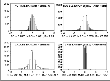
The normal distribution is a symmetric distribution with well-behaved tails and a single peak at the center of the distribution. By symmetric, we mean that the distribution can be folded about an axis so that the two sides coincide. That is, it behaves the same to the left and right of some center point. In this case, the median absolute deviation is a bit less than the standard deviation due to the downweighting of the tails. The range of a little less than 8 indicates the extreme values fall within about 4 standard deviations of the mean. If a histogram or normal probability plot indicates that your data are approximated well by a normal distribution, then it is reasonable to use the standard deviation as the spread estimator.
Comparing the double exponential and the normal histograms shows that the double exponential has a stronger peak at the center, decays more rapidly near the center, and has much longer tails. Due to the longer tails, the standard deviation tends to be inflated compared to the normal. On the other hand, the median absolute deviation is only slightly larger than it is for the normal data. The longer tails are clearly reflected in the value of the range, which shows that the extremes fall about 6 standard deviations from the mean compared to about 4 for the normal data.
The Cauchy distribution is a symmetric distribution with heavy tails and a single peak at the center of the distribution. The Cauchy distribution has the interesting property that collecting more data does not provide a more accurate estimate for the mean or standard deviation. That is, the sampling distribution of the means and standard deviation are equivalent to the sampling distribution of the original data. That means that for the Cauchy distribution the standard deviation is useless as a measure of the spread. From the histogram, it is clear that just about all the data are between about -5 and 5. However, a few very extreme values cause both the standard deviation and range to be extremely large. However, the median absolute deviation is only slightly larger than it is for the normal distribution. In this case, the median absolute deviation is clearly the better measure of spread.
Although the Cauchy distribution is an extreme case, it does illustrate the importance of heavy tails in measuring the spread. Extreme values in the tails can distort the standard deviation. However, these extreme values do not distort the median absolute deviation since the median absolute deviation is based on ranks. In general, for data with extreme values in the tails, the median absolute deviation or interquartile range can provide a more stable estimate of spread than the standard deviation.
The Tukey lambda distribution has a range limited to (-1/λ,1/λ). That is, it has truncated tails. In this case the standard deviation and median absolute deviation have closer values than for the other three examples which have significant tails.
Tukey and Mosteller defined two types of robustness where robustness is a lack of susceptibility to the effects of nonnormality.
- Robustness of validity means that the confidence intervals for a measure of the population spread (e.g., the standard deviation) have a 95 % chance of covering the true value (i.e., the population value) of that measure of spread regardless of the underlying distribution.
- Robustness of efficiency refers to high effectiveness in the face of non-normal tails. That is, confidence intervals for the measure of spread tend to be almost as narrow as the best that could be done if we knew the true shape of the distribution.
The median absolute deviation and the interquartile range are estimates of scale that have robustness of validity. However, they are not particularly strong for robustness of efficiency.
If histograms and probability plots indicate that your data are in fact reasonably approximated by a normal distribution, then it makes sense to use the standard deviation as the estimate of scale. However, if your data are not normal, and in particular if there are long tails, then using an alternative measure such as the median absolute deviation, average absolute deviation, or interquartile range makes sense. The range is used in some applications, such as quality control, for its simplicity. In addition, comparing the range to the standard deviation gives an indication of the spread of the data in the tails.
Since the range is determined by the two most extreme points in the data set, we should be cautious about its use for large values of N.
Tukey and Mosteller give a scale estimator that has both robustness of validity and robustness of efficiency. However, it is more complicated and we do not give the formula here.
