1.3. EDA Techniques
1.3.5. Quantitative Techniques
1.3.5.2. |
Confidence Limits for the Mean |
Interval Estimate for Mean
Confidence limits are expressed in terms of a confidence coefficient. Although the choice of confidence coefficient is somewhat arbitrary, in practice 90 %, 95 %, and 99 % intervals are often used, with 95 % being the most commonly used.
As a technical note, a 95 % confidence interval does not mean that there is a 95 % probability that the interval contains the true mean. The interval computed from a given sample either contains the true mean or it does not. Instead, the level of confidence is associated with the method of calculating the interval. The confidence coefficient is simply the proportion of samples of a given size that may be expected to contain the true mean. That is, for a 95 % confidence interval, if many samples are collected and the confidence interval computed, in the long run about 95 % of these intervals would contain the true mean.
-
\[ \bar{Y} \pm t_{1 - \alpha/2, \, N-1} \,\, \frac{s}{\sqrt{N}} \]
From the formula, it is clear that the width of the interval is controlled by two factors:
- As N increases, the interval gets narrower from
the
\(\sqrt{N}\) term.
That is, one way to obtain more precise estimates for the mean is to increase the sample size.
- The larger the sample standard deviation, the larger the confidence interval. This simply means that noisy data, i.e., data with a large standard deviation, are going to generate wider intervals than data with a smaller standard deviation.
| H0: | \( \mu = \mu_{0} \) |
| Ha: | \( \mu \neq \mu_{0} \) |
| Test Statistic: |
\( T = (\bar{Y} - \mu_{0})/(s/\sqrt{N}) \)
where \(\bar{Y}\), N, and s are defined as above. |
| Significance Level: | α. The most commonly used value for α is 0.05. |
| Critical Region: |
Reject the null hypothesis that the mean is a specified
value,
\(\mu_{0}\), if
|
N                          = 195
MEAN                       =   9.261460
STANDARD DEVIATION         =   0.022789
t1-0.025,N-1                 =   1.9723


LOWER LIMIT = 9.261460 - 1.9723*0.022789/√195

UPPER LIMIT = 9.261460 + 1.9723*0.022789/√195
Thus, a 95 % confidence interval for the mean is (9.258242, 9.264679).
H0:  μ = 5
Ha:  μ ≠ 5

Test statistic:  T = 2611.284
Degrees of freedom:  ν = 194
Significance level:  α = 0.05
Critical value:  t1-α/2,ν = 1.9723
Critical region:  Reject H0 if |T| > 1.9723
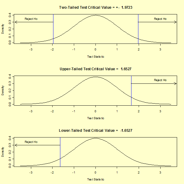
We reject the null hypotheses for our two-tailed t-test because the absolute value of the test statistic is greater than the critical value. If we were to perform an upper, one-tailed test, the critical value would be t1-α,ν = 1.6527, and we would still reject the null hypothesis.
The confidence interval provides an alternative to the hypothesis test. If the confidence interval contains 5, then H0 cannot be rejected. In our example, the confidence interval (9.258242, 9.264679) does not contain 5, indicating that the population mean does not equal 5 at the 0.05 level of significance.
In general, there are three possible alternative hypotheses and rejection regions for the one-sample t-test:
| Alternative Hypothesis | Rejection Region |
|---|---|
| Ha: μ ≠ μ0 | |T| > t1-α/2,ν |
| Ha: μ > μ0 | T > t1-α,ν |
| Ha: μ < μ0 | T < tα,ν |
The rejection regions for three posssible alternative hypotheses using our example data are shown in the following graphs.

- What is a reasonable estimate for the mean?
- How much variability is there in the estimate of the mean?
- Does a given target value fall within the confidence limits?
Confidence intervals for other location estimators such as the median or mid-mean tend to be mathematically difficult or intractable. For these cases, confidence intervals can be obtained using the bootstrap.

