TRIMMED MEAN STANDARD ERROR

TRIMMED MEAN STANDARD ERROR (LET)

Let Subcommand

Compute the standard error of the trimmed mean for a variable.

The mean is the sum of the observations divided by the number of observations. The mean can be heavily influenced by extreme values in the tails of a variable. The trimmed mean compensates for this by dropping a certain percentage of values on the tails. For example, the 50% trimmed mean is the mean of the values between the upper and lower quartiles. The 90% trimmed mean is the mean of the values after truncating the lowest and highest 5% of the values.

Mosteller and Tukey (see Reference section below) define two types of robustness:

1. resistance means that changing a small part, even by a large amount, of the data does not cause a large change in the estimate

2. robustness of efficiency means that the statistic has high efficiency in a variety of situations rather than in any one situation. Efficiency means that the estimate is close to optimal estimate given that we know what distribution that the data comes from. A useful measure of efficiency is:
   Efficiency = (lowest variance feasible)/ (actual variance)

Many statistics have one of these properties. However, it can be difficult to find statistics that are both resistant and have robustness of efficiency.

For location estimaors, the mean is the optimal estimator for Gaussian data. However, it is not resistant and it does not have robustness of efficiency. The trimmed mean estimator is both resistant and robust of efficiency.

The standard error of the trimmed mean can be used to estimate the uncertainty of the trimmed mean estimate (and to create confidence intervals). The trimmed mean standard error is defined as:

\( se_{t} = \frac{s_{w}}{(1 - (\gamma_1 + \gamma_2))\sqrt{n}} \)

where s_w is the Winsorized standard deviation (enter HELP WINSORIZED STANDARD DEVIATION for details), \( \gamma_1 \) is the lower trimming fraction, \( \gamma_2 \) is the upper trimming fraction, and n is the sample size.

Tukey and Mclaughlin suggest the following confidence interval for the trimmed mean:

\( \bar{X}_{t} = t_{(1-\alpha/2,n-2g-1)} se_{t} \)

where alpha is the desired significance level, t is the student t-distribution, and \( g = [\gamma n] \) (the integer portion of the trimming fraction times the sample size). Note that we are assuming equal trimming on both tails (\( \gamma \) = .10 means we trim 10% on both tails).

An alternative method for confidence intervals is to use the BOOTSTRAP TRIMMED MEAN PLOT command and use appropriate percentiles of the generated bootstrap trimmed mean values. Wilcox suggests a refinement of the standard bootstrap, which he calls he percentile t bootstrap, which has better performance than the standard bootstrap. Dataplot does not currently support this refinement.

LET <par> = TRIMMED MEAN STANDARD ERROR <y1>
                            <SUBSET/EXCEPT/FOR qualification>
where <y1> is the response variable;
              <par> is a parameter where the computed trimmed mean standard error is stored;
and where the <SUBSET/EXCEPT/FOR qualification> is optional.

LET A = TRIMMED MEAN STANDARD ERROR Y1
LET A = TRIMMED MEAN STANDARD ERROR Y1 SUBSET TAG > 2

The analyst must specify the percentages to trim in each tail. This is done by defining the internal variables P1 (the lower tail) and P2 (the upper tail). For example, to trim 10% off each tail, do the following:
LET P1 = 10
LET P2 = 10
LET A = TRIMMED MEAN STANDARD ERROR Y

Dataplot statistics can be used in 20+ commands. For details, enter
HELP STATISTICS

None

None

TRIMMED MEAN	= Compute the trimmed mean.
MEAN	= Compute the mean.
WINSORIZED MEAN	= Compute the Winsorized mean.
MEDIAN	= Compute the median.
STATISTIC PLOT	= Generate a statistic versus group plot for a given statistic.
BOOTSTRAP PLOT	= Generate a bootstrap plot for a given statistic.
INFLUENCE CURVE	= Generate an influence curve for a given statistic.

Rand Wilcox (1997), "Introduction to Robust Estimation and Hypothesis Testing", Academic Press.

Tukey and McLaughlin, "Less Vunerable Confidence and Significance Procedures for Location Based on a Single Sample: Trimming/Winsorization", Sankhya A, 25, pp. 331-352.

Mosteller and Tukey (1977), "Data Analysis and Regression: A Second Course in Statistics", Addison-Wesley, pp. 203-209.

Robust Data Analysis

2002/07

 
LET Y1 = NORMAL RANDOM NUMBERS FOR I = 1 1 100
LET Y2 = LOGISTIC RANDOM NUMBERS FOR I = 1 1 100
LET Y3 = CAUCHY RANDOM NUMBERS FOR I = 1 1 100
LET Y4 = DOUBLE EXPONENTIAL RANDOM NUMBERS FOR I = 1 1 100
LET A1 = TRIMMED MEAN STANDARD ERROR Y1
LET A2 = TRIMMED MEAN STANDARD ERROR Y2
LET A3 = TRIMMED MEAN STANDARD ERROR Y3
LET A4 = TRIMMED MEAN STANDARD ERROR Y4
    

MULTIPLOT 2 2
MULTIPLOT CORNER COORDINATES 0 0 100 100
MULTIPLOT SCALE FACTOR 2
X1LABEL DISPLACEMENT 12
.
LET Y1 = NORMAL RANDOM NUMBERS FOR I = 1 1 200
LET Y2 = CAUCHY RANDOM NUMBERS FOR I = 1 1 200
LET P1 = 10
LET P2 = 10
.
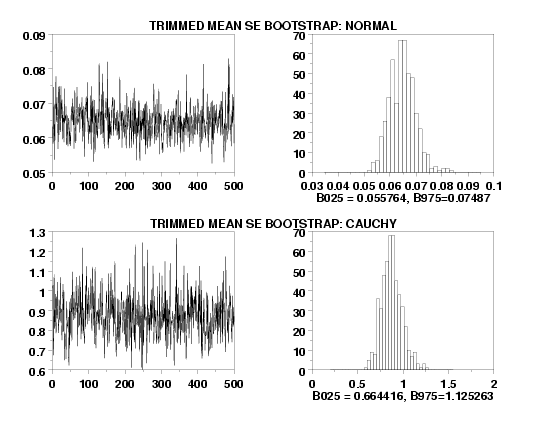
BOOTSTRAP SAMPLES 500
BOOTSTRAP TRIMMED MEAN STANDARD ERROR PLOT Y1
X1LABEL B025 = ^B025, B975=^B975
HISTOGRAM YPLOT
X1LABEL
.
BOOTSTRAP BIWEIGHT MIDVARIANCE PLOT Y1
X1LABEL B025 = ^B025, B975=^B975
HISTOGRAM YPLOT
.
END OF MULTIPLOT
.
JUSTIFICATION CENTER
MOVE 50 46
TEXT TRIMMED MEAN SE BOOTSTRAP: CAUCHY
MOVE 50 96
TEXT TRIMMED MEAN SE BOOTSTRAP: NORMAL