PEAKS OF FREQUENCY TABLE

PEAKS OF FREQUENCY TABLE (LET)

Let Subcommand

Bin (i.e., create a frequency table) a response variable and then thin the frequency table by extracting the peaks.

Binning a data variable means to divide it into classes and compute the frequency for each class. This is the numerical equivalent of a histogram.

Peaks are determined as follows:

1. Compute the difference of the frequency counts.

2. Where the differences change sign indicates a peak.

Also, you can specify that relative frequencies rather than counts be computed. The command

SET RELATIVE HISTOGRAM <AREA/PERCENT>

can be used to specify whether relative frequencies are computed so that the area sums to 1 or so that frequencies sum to 1. The first option, which is the default, is useful for when using the relative binning as an estimate of a probability distribution. The second option is useful when you want to see what percentage of the data falls in a given class.

LET <y2> <x2> = PEAKS OF FREQUENCY TABLE <y>
                        <SUBSET/EXCEPT/FOR qualification> where <y> is the response variable;
            <y2> is a variable where the computed counts (or frequencies) are stored;
            <x2> is a variable where the computed bin mid-points are stored;
and where the <SUBSET/EXCEPT/FOR qualification> is optional.

This syntax is used for the case where the frequencies are expressed as raw counts.

LET <y2> <x2> = RELATIVE PEAKS OF FREQUENCY TABLE <y>
                        <SUBSET/EXCEPT/FOR qualification>
where <y> is the response variable;
            <y2> is a variable where the computed counts (or frequencies) are stored;
            <x2> is a variable where the computed bin mid-points are stored;
and where the <SUBSET/EXCEPT/FOR qualification> is optional.

This syntax is used for the case where the frequencies are expressed as relative frequencies.

LET Y2 X2 = PEAKS OF FREQUENCY TABLE Y
LET Y2 X2 = PEAKS OF FREQUENCY TABLE Y SUBSET TAG > 2
LET Y2 X2 = RELATIVE PEAKS OF FREQUENCY TABLE Y

As with the histogram, you can use the CLASS WIDTH, CLASS LOWER, and CLASS UPPER commands to override these defaults.

By default, DATAPLOT uses a class width of 0.3 times the standard deviation of the variable. A number of alternative choices for class width can be set with the command

SET HISTOGRAM CLASS WIDTH

Enter HELP HISTOGRAM CLASS WIDTH for details.

None

None

BINNED	= Compute a frequency table.
COMBINE FREQUENCY TABLE	= Combine low frequency classes in a
HISTOGRAM	= Generate a histogram.
CLASS WIDTH	= Set class widths for histograms and other related commands.
HISTOGRAM CLASS WIDTH	= Set class widths for histograms and other related commands.

Data Analysis

2008/4

 
let u1 = 0
let sd1 = 1
let u2 = 5
let sd2 = 3
let p = 0.6
let y = normal mixture rand numb for i = 1 1 500
.
set write decimals 4
let y2 x2 = binned y
print x2 y2
.
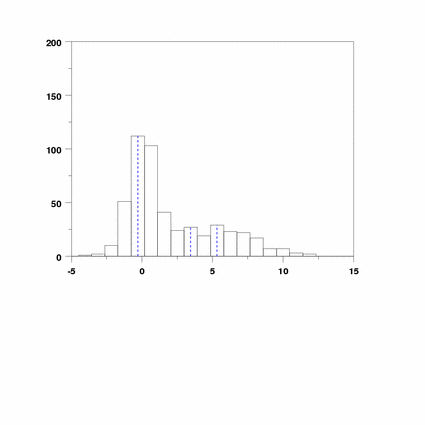
let y3 x3 = peaks of frequency table y
print x3 y3
.
xlimits -5 15
histogram y
.
line color blue
line dash
line thickness 0.2
let ycoor1 = 0
let npeak = size x3
.
loop for k = 1 1 npeak
    let xtemp = x3(k)
    let ytemp = y3(k)
    drawdata xtemp ycoor1 xtemp ytemp
end of loop
    

The following output is generated.

 VARIABLES--X2             Y2

        -4.0351         1.0000
        -3.0993         2.0000
        -2.1636        10.0000
        -1.2278        51.0000
        -0.2921       112.0000
         0.6437       103.0000
         1.5795        41.0000
         2.5152        24.0000
         3.4510        27.0000
         4.3868        19.0000
         5.3225        29.0000
         6.2583        23.0000
         7.1941        22.0000
         8.1298        17.0000
         9.0656         7.0000
        10.0014         7.0000
        10.9371         3.0000
        11.8729         2.0000

 VARIABLES--X3             Y3

        -0.2921       112.0000
         3.4510        27.0000
         5.3225        29.0000