
|
|
HEDGES GName:
BIAS CORRECTED HEDGES G (LET) COHENS D (LET) GLASS G (LET)
with \( \bar{y}_{1} \), \( \bar{y}_{2} \), and \( s_{p} \) denoting the mean of sample 1, the mean of sample 2, and the pooled standard deviation, respectively. The formula for the pooled standard deviation is
with \( s_{1} \) and \( n_{1} \) denoting the standard deviation and number of observations for sample 1, respectively, and \( s_{2} \) and \( n_{2} \) denoting the standard deviation and number of observations for sample 2, respectively. The Hedge's g statistic expresses the difference of the means in units of the pooled standard deviation. For small samples, the following bias correction is recommended
where \( n = n_{1} + n_{2} \). This bias correction is typically recommended when n < 50. NOTE:
The term being approximated is
where
with \( \Gamma \) denoting the Gamma function. Running a comparison indicated that Hedge's original approximation is more accurate than that given by Durlak. The 2018/08 version of Dataplot modified the bias correction to use the original J function with Gamma functions for \( n_1 + n_2 \le 40 \) and to use Hedge's original approximation otherwise. Hedge's g is similar to the Cohen's d statistic and the Glass g statistic. The difference is what is used for the estimate of the pooled standard deviation. The Hedge's g uses a sample size weighted pooled standard deviation while Cohen's d uses
These statistic are typically used to compare an experimental sample to a control sample. The Glass g statistic uses the standard deviation of the control sample rather than the pooled standard deviation. His argument for this is that experimental samples with very different standard deviations can result in significant differences in the g statistic for equivalent differences in the mean. So the Glass g statistic measures the difference in means in units of the control sample standard deviation. Hedge's g, Cohen's d, and Glass's g are interpreted in the same way. Cohen recommended the following rule of thumb
However, Cohen did suggest caution for this rule of thumb as the meaning of small, medium and large may vary depending on the context of a particular study. The Hedge's g statistic is generally preferred to Cohen's d statistic. It has better small sample properties and has better properties when the sample sizes are signigicantly different. For large samples where \( n_{1} \) and \( n_{2} \) are similar, the two statistics should be almost the same. The Glass g statistic may be preferred when the standard deviations are quite different. In many cases, there are multiple experimental groups being compared to the control. This could be either a separate control sample for each experiment (e.g., we are comparing effect sizes from different experiments) or a common control (e.g., different laboratories are measuring identical material and are being compared to a reference measurement). In these cases, you can compute the Hedge's g (or Glass's g or Cohen's d) for each experiment relative to its control group. You can then obtain an "overall" value of the statistic by averaging these individual statistics.
<SUBSET/EXCEPT/FOR qualification> where <y1> is the first response variable; <y2> is the second response variable; <par> is a parameter where the computed Hedge's g statistic is stored; and where the <SUBSET/EXCEPT/FOR qualification> is optional. This syntax computes Hedge's g statistic without the bias correction.
<SUBSET/EXCEPT/FOR qualification> where <y1> is the first response variable; <y2> is the second response variable; <par> is a parameter where the computed bias corrected Hedge's g statistic is stored; and where the <SUBSET/EXCEPT/FOR qualification> is optional. This syntax computes the Hedge's g statistic with the bias correction.
<SUBSET/EXCEPT/FOR qualification> where <y1> is the first response variable; <y2> is the second response variable; <par> is a parameter where the computed Glass's g statistic is stored; and where the <SUBSET/EXCEPT/FOR qualification> is optional. This syntax computes Glass's g statistic. The <y2> variable will be treated as the "control" sample. That is, the standard deviation of <y2> will be used as the pooled standard deviation.
<SUBSET/EXCEPT/FOR qualification> where <y1> is the first response variable; <y2> is the second response variable; <par> is a parameter where the computed Cohen's d statistic is stored; and where the <SUBSET/EXCEPT/FOR qualification> is optional. This syntax computes Cohen's d statistic.
LET A = BIAS CORRECTED HEDGES G Y1 Y2 LET A = BIAS CORRECTED HEDGES G Y1 Y2 SUBSET Y1 > 0 LET A = GLASS G Y1 Y2 LET A = COHENS D Y1 Y2
Cohen (1977), "Statistical Power Analysis for the Behavioral Sciences", Routledge. Glass (1976), "Primary, Secondary, and Meta-Analysis of Research", Educational Researcher, Vol. 5, pp. 3-8. Durlak (2009), "How to Select, Calculate, and Interpret Effect Sizes", Journal of Pediatric Psychology, Vol. 34, No. 9, pp. 917-928. Hedges and Olkin (1985), "Statistical Methods for Meta-Analysis", New York: Academic Press.
SKIP 25
READ IRIS.DAT Y1 TO Y4 X
.
LET A = HEDGES G Y1 Y2
TABULATE HEDGES G Y1 Y2 X
.
LABEL CASE ASIS
TITLE CASE ASIS
Y1LABEL Hedge's G Statistic
X1LABEL Group
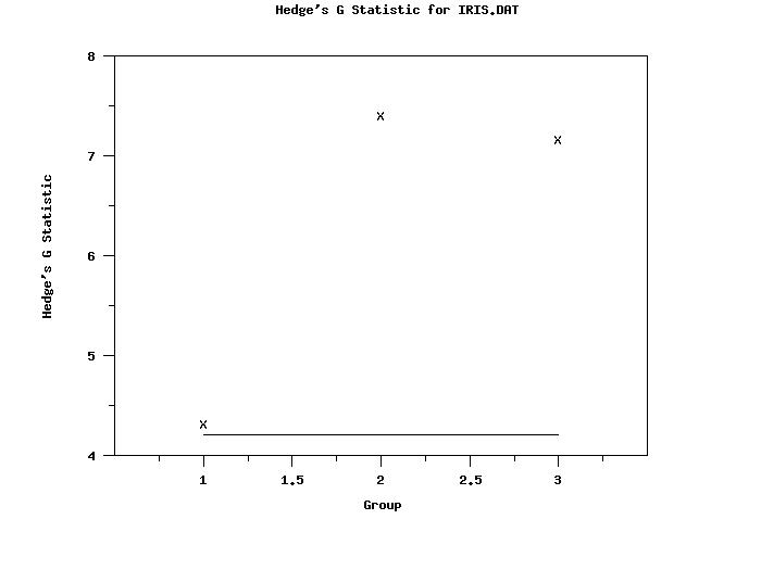
TITLE Hedge's G Statistic for IRIS.DAT
X1TIC MARK OFFSET 0.5 0.5
TIC MARK OFFSET UNITS DATA
CHAR X
LINE BLANK
HEDGES G PLOT Y1 Y2 X
.
Y1LABEL Hedge's G Statistic
X1LABEL Group
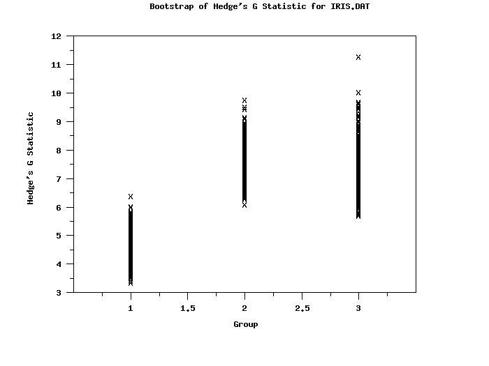
TITLE Bootstrap of Hedge's G Statistic for IRIS.DAT
CHAR X ALL
LINE BLANK ALL
BOOTSTRAP SAMPLES 1000
BOOTSTRAP HEDGES G PLOT Y1 Y2 X
The following output is generated
            Cross Tabulate HEDGES G

(Response Variables: Y1       Y2      )
---------------------------------------------
       X          |          HEDGES G
---------------------------------------------
  0.1000000E+01   |     0.4311260E+01
  0.2000000E+01   |     0.7412040E+01
  0.3000000E+01   |     0.7168413E+01
            Bootstrap Analysis for the HEDGES G

Response Variable One: Y1
Response Variable Two: Y2
Group ID Variable One (X       ):          1.000000

Number of Bootstrap Samples:             1000
Number of Observations:                  50
Mean of Bootstrap Samples:                 4.389604
Standard Deviation of Bootstrap Samples:  0.4288846
Median of Bootstrap Samples:               4.335823
MAD of Bootstrap Samples:                 0.2615915
Minimum of Bootstrap Samples:              3.342993
Maximum of Bootstrap Samples:              6.389001


Percent Points of the Bootstrap Samples
-----------------------------------
  Percent Point               Value
-----------------------------------
            0.1    =   3.343002
            0.5    =   3.511410
            1.0    =   3.546756
            2.5    =   3.687836
            5.0    =   3.798257
           10.0    =   3.910058
           20.0    =   4.037920
           50.0    =   4.335823
           80.0    =   4.705708
           90.0    =   4.947669
           95.0    =   5.174219
           97.5    =   5.409715
           99.0    =   5.681841
           99.5    =   5.823756
           99.9    =   6.388623


            Percentile Confidence Interval for Statistic

------------------------------------------
  Confidence          Lower          Upper
 Coefficient          Limit          Limit
------------------------------------------
       50.00   4.087805       4.619201
       75.00   3.934208       4.869211
       90.00   3.798257       5.174219
       95.00   3.687836       5.409715
       99.00   3.511410       5.823756
       99.90   3.342993       6.389001
------------------------------------------


Response Variable One: Y1
Response Variable Two: Y2
Group ID Variable One (X       ):          2.000000

Number of Bootstrap Samples:             1000
Number of Observations:                  50
Mean of Bootstrap Samples:                 7.537408
Standard Deviation of Bootstrap Samples:  0.5465833
Median of Bootstrap Samples:               7.499111
MAD of Bootstrap Samples:                 0.3508403
Minimum of Bootstrap Samples:              6.092766
Maximum of Bootstrap Samples:              9.751977


Percent Points of the Bootstrap Samples
-----------------------------------
  Percent Point               Value
-----------------------------------
            0.1    =   6.092945
            0.5    =   6.287894
            1.0    =   6.397113
            2.5    =   6.541644
            5.0    =   6.668351
           10.0    =   6.842498
           20.0    =   7.102805
           50.0    =   7.499111
           80.0    =   7.976231
           90.0    =   8.257037
           95.0    =   8.490531
           97.5    =   8.726730
           99.0    =   8.898412
           99.5    =   9.116481
           99.9    =   9.751736


            Percentile Confidence Interval for Statistic

------------------------------------------
  Confidence          Lower          Upper
 Coefficient          Limit          Limit
------------------------------------------
       50.00   7.171687       7.894311
       75.00   6.920084       8.177537
       90.00   6.668351       8.490531
       95.00   6.541644       8.726730
       99.00   6.287894       9.116481
       99.90   6.092766       9.751977
------------------------------------------


Response Variable One: Y1
Response Variable Two: Y2
Group ID Variable One (X       ):          3.000000

Number of Bootstrap Samples:             1000
Number of Observations:                  50
Mean of Bootstrap Samples:                 7.338842
Standard Deviation of Bootstrap Samples:  0.6960418
Median of Bootstrap Samples:               7.310299
MAD of Bootstrap Samples:                 0.4584347
Minimum of Bootstrap Samples:              5.688356
Maximum of Bootstrap Samples:              11.27284


Percent Points of the Bootstrap Samples
-----------------------------------
  Percent Point               Value
-----------------------------------
            0.1    =   5.688367
            0.5    =   5.747268
            1.0    =   5.929775
            2.5    =   6.122410
            5.0    =   6.271287
           10.0    =   6.488546
           20.0    =   6.749534
           50.0    =   7.310299
           80.0    =   7.873042
           90.0    =   8.208357
           95.0    =   8.487544
           97.5    =   8.823580
           99.0    =   9.252583
           99.5    =   9.609171
           99.9    =   11.27161


            Percentile Confidence Interval for Statistic

------------------------------------------
  Confidence          Lower          Upper
 Coefficient          Limit          Limit
------------------------------------------
       50.00   6.862967       7.771134
       75.00   6.543979       8.090032
       90.00   6.271287       8.487544
       95.00   6.122410       8.823580
       99.00   5.747268       9.609171
       99.90   5.688356       11.27284
------------------------------------------


Response Variable One: Y1
Response Variable Two: Y2
Group ID Variable One (All Data):

Number of Bootstrap Samples:             1000
Number of Observations:                  150
Mean of Bootstrap Samples:                 6.421951
Standard Deviation of Bootstrap Samples:   1.547468
Median of Bootstrap Samples:               7.007179
MAD of Bootstrap Samples:                 0.8567694
Minimum of Bootstrap Samples:              3.342993
Maximum of Bootstrap Samples:              11.27284


Percent Points of the Bootstrap Samples
-----------------------------------
  Percent Point               Value
-----------------------------------
            0.1    =   3.409331
            0.5    =   3.625963
            1.0    =   3.741478
            2.5    =   3.852497
            5.0    =   3.968823
           10.0    =   4.131668
           20.0    =   4.447991
           50.0    =   7.007179
           80.0    =   7.739732
           90.0    =   8.062719
           95.0    =   8.351421
           97.5    =   8.614502
           99.0    =   8.894499
           99.5    =   9.203490
           99.9    =   9.751902


            Percentile Confidence Interval for Statistic

------------------------------------------
  Confidence          Lower          Upper
 Coefficient          Limit          Limit
------------------------------------------
       50.00   4.617406       7.610766
       75.00   4.210556       7.962787
       90.00   3.968823       8.351421
       95.00   3.852497       8.614502
       99.00   3.625963       9.203490
       99.90   3.347339       10.65474
------------------------------------------
|
Privacy
Policy/Security Notice
NIST is an agency of the U.S.
Commerce Department.
Date created: 07/26/2017 | |||||||||||||||||||||||||||||||