TUKEY MEAN-DIFFERENCE PLOT

TUKEY MEAN-DIFFERENCE PLOT

Graphics Command

Generates a Tukey mean-difference plot.

The Tukey mean-difference plot is an adaption of the quantile-quantile plot.

A quantile-quantile plot (or q-q plot) is a graphical data analysis technique for comparing the distributions of 2 data sets. The quantile-quantile plot is a graphical alternative for the various classical 2-sample tests (e.g., t for location, F for dispersion).

The plot consists of the following:

Vertical axis = estimated quantiles from data set 1;
Horizontal axis = estimated quantiles from data set 2.


The "quantiles" of a distribution are the distribution's "percent points" (e.g., .5 quantile = 50% point = median). The advantage of the quantile-quantile plot is 2-fold:

1. the sample sizes do not need to be identical;
2. many distributional aspects can be simultaneously tested. For example, shifts in location, shifts in dispersion, changes in symmetry/skewness, outliers, etc.

The quantile-quantile plot has 2 components:

1. the quantile points themselves;
2. a 45 degree reference line.

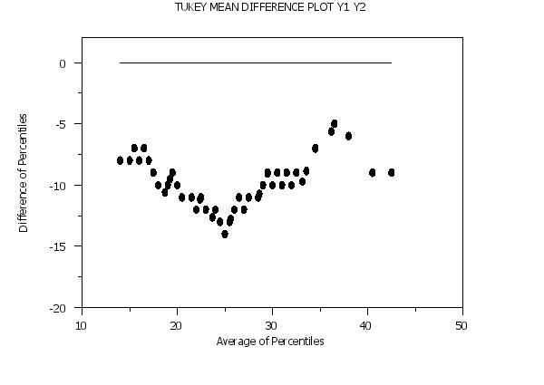
Given a q-q plot, assume its y coordinates are in T(i) and its x coordinates are in D(i), then the Tukey mean-difference is defined as:

Vertical axis = T(i) - D(i);
Horizontal axis = (T(i) + D(i)/2.


The Tukey mean-difference plot also plots a horizontal reference line at zero.

That is, it plots the difference of the quantiles against their average. The advantage of the Tukey mean-difference compared to the q-q plot is that it converts interpretation of the differences around a 45 degree diagonal line to interpretation of differences around a horizontal zero line. However, the Tukey mean-difference plot should only be applied if the two variables are on a common scale.

Like usual, the appearance of the 2 components is controlled by the first 2 settings of the CHARACTERS and LINES commands. It is typical for the response points to be represented as some character, say X's, with no connecting line, and the reference line as a connected line with no character. This is demonstrated in the sample program below.

TUKEY MEAN DIFFERENCE PLOT <y1> <y2>
                        <SUBSET/EXCEPT/FOR qualification>
where <y1> is the first response variable;
            <y2> is the second response variable;
and where the <SUBSET/EXCEPT/FOR qualification> is optional.

HIGHLIGHT TUKEY MEAN DIFFERENCE PLOT <y1> <y2> <tag>
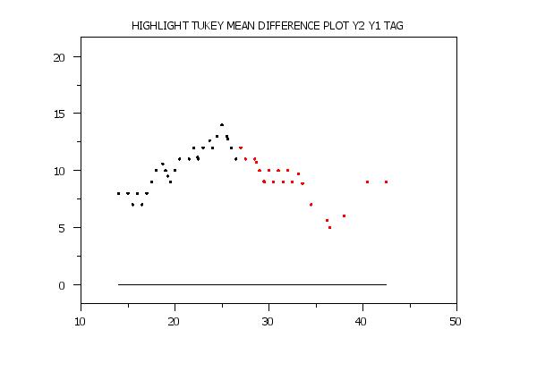
                        <SUBSET/EXCEPT/FOR qualification>
where <y1> is the first response variable;
            <y2> is the second response variable;
            <tag> is the group-id variable that defines the highlighting;
and where the <SUBSET/EXCEPT/FOR qualification> is optional.

This syntax can be used to plot different plot points with different attributes. For example, it can used to highlight groups in the data or to emphasize the extremes.

TUKEY MEAN DIFFERENCE PLOT Y1 Y2
TUKEY MEAN DIFFERENCE PLOT RUN1 RUN2
TUKEY MEAN DIFFERENCE PLOT BATCH1 BATCH2
TUKEY MEAN DIFFERENCE PLOT Y1 Y2 SUBSET AUTO 4
TUKEY MEAN DIFFERENCE PLOT Y1 Y2 SUBSET STATE 25

One of the distributions can be a theoretical distribution. For example, the following program generates a Tukey mean-difference plot of a data set against a normal distribution.
LET Y1 = NORMAL RANDOM NUMBERS FOR I = 1 1 100
LET X = SEQUENCE .01 .01 .99
LET Y2 = NORPPF(X)
TUKEY MEAN DIFFERENCE PLOT Y1 Y2


This same technique can be used other distributions (use the appropriate PPF function).

For large data sets, it may be impractical to generate the plot for each individual point. As an alternative, you can generate the plot for a user specified number of quantiles. To do this, enter the command
SET QUANTILE QUANTILE PLOT NUMBER OF PERCENTILES ...
            <value>

where <value> specifies the desired number of quantiles. This is demonstrated in the Program 2 example below.

None

TUKEY M-D PLOT is a synonym for TUKEY MEAN DIFFERENCE PLOT.

CHARACTERS	= Sets the type for plot characters.
LINES	= Sets the type for plot lines.
QUANTILE-QUANTILE PLOT	= Generates a q-q plot.
BOX PLOT	= Generates a box plot.
BIHISTOGRAM	= Generates a bihistogram.
PLOT	= Generates a data or function plot.
PROBABILITY PLOT	= Generates a probability plot.
T-TEST	= Carries out a 2-sample t test.
F-TEST	= Carries out a 2-sample F test.

Cleveland, William S. (1993), "Visualizing Data", Hobart Press,

Chambers, Cleveland, Kleiner, and Tukey (1983), "Graphical Methods of Data Analysis", Wadsworth, pp. 48-57.

Exploratory Data Analysis

2000/1

 
SKIP 25
READ AUTO83B.DAT Y1 Y2
.
DELETE Y2 SUBSET Y2 < 0
LINE BLANK SOLID
CHARACTER CIRCLE BLANK
CHARACTER FILL ON OFF
TIC OFFSET UNITS DATA
YTIC OFFSET 0 2
TITLE AUTOMATIC
LABEL CASE ASIS
Y1LABEL Difference of Percentiles
X1LABEL Average of Percentiles
TUKEY MEAN DIFFERENCE PLOT Y1 Y2
    

 
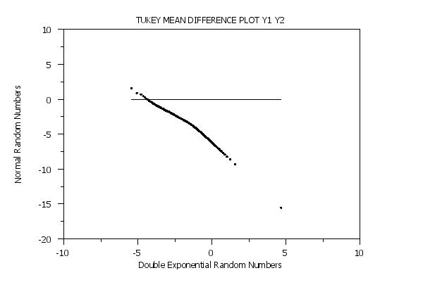
LET Y1 = NORMAL RANDOM NUMBER FOR I = 1 1 1000000
LET Y2 = DOUBLE EXPONENTIAL RANDOM NUMBER FOR I = 1 1 1000000
.
LINE BLANK SOLID
CHARACTER CIRCLE BLANK
CHARACTER FILL ON OFF
CHARACTER HW 0.5 0.375
TITLE AUTOMATIC
TITLE OFFSET 2
LABEL CASE ASIS
Y1LABEL Normal Random Numbers
X1LABEL Double Exponential Random Numbers
.
SET QUANTILE QUANTILE PLOT NUMBER OF PERCENTILES 1000
TUKEY MEAN DIFFERENCE PLOT Y1 Y2
    

 
SKIP 25
READ AUTO83B.DAT Y1 Y2
DELETE Y2 SUBSET Y2 < 0
.
LINE BLANK BLANK SOLID
CHARACTER CIRCLE CIRCLE BLANK
CHARACTER FILL ON ON OFF
CHARACTER HW 0.5 0.375 ALL
CHARACTER COLOR BLACK RED
TITLE AUTOMATIC
TITLE OFFSET 2
TIC MARK OFFSET UNITS SCREEN
YTIC MARK OFFSET 5 5
.
LET N2 = SIZE Y2
LET TAG = 1 FOR I = 1 1 N2
LET TAG = 2 SUBSET Y2 > 32
.
HIGHLIGHT TUKEY MEAN DIFFERENCE PLOT Y2 Y1 TAG