FUNCTION BLOCK

FUNCTION BLOCK

Analysis Command

Defines a function via a group of Dataplot commands.

Dataplot allows users to define their own functions using a Fortran-like syntax. For example,
LET FUNCTION F = (x-a0)/a1
LET FUNCTION F = X1**2
LET FUNCTION G = P*(L-X)/(E*I)


User defined functions can be used in subsequent commands such as PLOT and LET (basically any place that a built-in Dataplot function can be used).

Although Dataplot functions can be powerful, they do have some important limitations for some applications. In particular, Dataplot functions are evaluated on a "row by row" basis. Many statistical applications involve root finding or optimization for functions that involve sums of some kind.

Function blocks were introduced to address this limitation. Function blocks allow you to define functions using various Dataplot LET subcommands.

Function blocks are created using the CAPTURE syntax. For example,

CAPTURE FUNCTION BLOCK ONE F A G
LET C2 = 1/G
LET Y2 = Y**G
LET W = Y2*Z
LET A1 = SUM W
LET A2 = SUM Y2
LET A = C2 - (A1/A2) + C1
END OF CAPTURE


The function block contains the following components

1. CAPTURE FUNCTION BLOCK - this initiates the creation of the function block. The CAPTURE command is typically used to direct Dataplot output to a file. However, in this case it saves the specified commands in an internal structure that can be accessed later.

2. ONE - up to three function blocks can be defined. In this example, "ONE" specifies that this is function block one. You can redefine these three function blocks as often as you need in a Dataplot session.

3. F - this is the name of the function block. This is the name that will be used to execute the function block in subsequent commands. This follows the rules for other Dataplot names (i.e., up to eight alphanumeric characters).

4. A - this is name of the parameter that will contain the response for the function block. This is the value that is typically defined in the last line of the function block. In this example, the response is a parameter. However, in some cases, it may be a variable.

5. G - this is a parameter that is being updated by the function block. In this case, we have only one parameter. In some cases, you may have more than one parameter.

   For example, in an optimization problem, you may be looking for the value of the parameter that minimizes (or maximizes) the value of a function. The OPTIMIZE command will search over the specified parameter (G in this example) to find the optimal value.

   Parameters that remain fixed do not need to be specified on the CAPTURE command.

   Up to 20 parameters can be specified for a given function block.

The following Dataplot commands can be included in a function block:

1. LET ... = PATTERN ...
2. LET ... = DATA ...
3. LET ... = ... RANDOM NUMBERS ...
4. ARITHMETIC OPERATIONS
5. STATISTIC LET SUB-COMMANDS
6. MATH LET SUB-COMMANDS

   The following MATH LET sub-commands are not allowed:

   • MATRIX sub-commands
   • DERIVATIVE
   • NUMERICAL DERIVATIVE
   • INTEGRAL
   • RUNGE-KUTTA
   • OPTIMIZE
   • ROOTS

The arithmetic operations and statistics LET sub-commands are of particular interest. Commands that are not supported are not added to the function block during the CAPTURE operation. Up to 30 commands can be saved to a given function block.

Currently, function blocks can be used with the following commands:

1. PLOT <function>
2. 3D-PLOT <function>
3. LET ... = ROOTS ...
4. LET ... = OPTIMIZE ...
5. LET ... = INTEGRAL ...
6. LET ... = NUMERICAL DERIVATIVE ...

CAPTURE FUNCTION BLOCK <one/two/three> <name> <resp> <parameter list>
where <one/two/three> specifies which function block is being created;
            <name> is the name of the function block;
            <resp> is the name of parameter or a variable that is the result of the function block;
and       <parameter list> is a list of 1 to 20 parameter names.

This syntax is used to create the contents of a function block.

LIST FUNCTION BLOCK <one/two/three>
where <one/two/three> specifies which function block is being listed.

This syntax is used to list the contents of a function block.

capture function block one f a sigma gamma
let c1 = n*(log(gamma) - gamma*log(sigma))
let c2 = (gamma - 1)*ylogsum
let y2 = (y/sigma)**gamma
let c3 = sum y2
let a = c1 + c2 - c3
end of capture

Error checking (e.g., matching parenthesis, valid number of arguments for a built-in function) is performed when the function block is evaluated, not when it is created.

There may be cases where you cannot create the needed function even with the FUNCTION BLOCK command. The LET ... = EXECUTE ... command can be used to run an external prorgram. That is, your function block can use the EXECUTE command to compute the desired function. You can create the external program in whatever language is most convenient for your application. The basic requirement is that the resulting external file can be run from the command line and that it can read from standard input and write to standard output.

None

None

LET	= Carries out a variety of operations on variables, parameters, and functions.
LET FUNCTION	= Define a function.
EXECUTE	= Run an external program.
CAPTURE	= Direct Dataplot output to an external file.
STATISTIC BLOCK	= Define a statistic block.
PLOT	= Plot a function of one variable.
3D-PLOT	= Plot a function of two variables.
ROOTS	= Find the roots of a univariate function.
OPTIMIZE	= Find the maximum (or minimum) of a function.
INTEGRAL	= Find the integral of a function.
NUMERICAL DERIVATIVE	= Find the numerical derivative of a function.

Mathematics

2015/11

 
. Purpose:  Demonstrate the use of function blocks
.
. Step 1:   Read the data
.
skip 25
read weibbury.dat y
skip 0
.
. Step 2:   Define the function block
.
let n = size y
let z = log(y)
let zsum = sum z
let c1 = zsum/n
.
capture function block one f a g
let c2 = 1/g
let y2 = y**g
let w  = y2*z
let a1 = sum w
let a2 = sum y2
let a  = c2 - (a1/a2) + c1
end of capture
.
list function block one
    

The following output is generated.

CONTENTS OF FUNCTION BLOCK ONE:
let c2 = 1/g
let y2 = y**g
let w  = y2*z
let a1 = sum w
let a2 = sum y2
let a  = c2 - (a1/a2) + c1
NAME FOR FUNCTION BLOCK ONE: F
PARAMETER LIST FOR FUNCTION BLOCK ONE:
PARAMETER  1: G
RESPONSE PARAMETER/VARIABLE: A
    

.
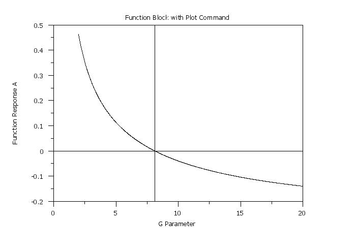
. Step 3:   Plot the function
.
title offset 2
title case asis
label case ais
y1label Function Response A
x1label G Parameter 
title Function Block with Plot Command
plot f for g = 2  0.01 20
delete g
.
. Step 3:   Now use it to solve an equation
.
let yroot = roots f wrt g for g = 2  20
    

The following output is generated.

 ROOTS OF AN EQUATION
       ROOT VARIABLE                     = G
       SPECIFIED LOWER LIMIT OF INTERVAL =         2.0000000000
       SPECIFIED UPPER LIMIT OF INTERVAL =        20.0000000000
  
       NUMBER OF ROOTS FOUND IN INTERVAL =        1
  
 ROOT     1 =    8.117599
    

let ztemp = yroot(1)
.
line dash
drawsdsd 15 0 85 0
drawdsds ztemp 20 ztemp 90
    



.
let yinte = integral f wrt g for g = 2  6
print yinte
    

The following output is generated.

 PARAMETERS AND CONSTANTS--

     YINTE   --  0.8159837E+00
    

.
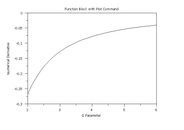
let yder = numerical derivative f wrt g for g = 4.2
    

The following output is generated.

 AT X0 =    4.200000     THE DERIVATIVE VALUE  =  -0.7183620E-01
 (WITH ESTIMATED ERROR =   0.8401624E-04)
  
  
 THE COMPUTED VALUE OF THE CONSTANT   YDER     =  -0.7183620E-01
    

let gtemp = sequence 2 0.05 6
let yd = numerical derivative f wrt gtemp
y1label Numerical Derivative
plot yd gtemp
    

 
. Purpose:  Demonstrate the use of function blocks in univariate
.           optimization
.
. Step 1:   Read the data
.
skip 25
read weibbury.dat y
skip 0
.
. Step 2:   Define the function block
.
set optimization maximum
capture function block one f a gamma
let a  = weibull ppcc statistic y
end of capture
.
list function block one
    

The following output is generated.

 CONTENTS OF FUNCTION BLOCK ONE:
 let a  = weibull ppcc statistic y
 NAME FOR FUNCTION BLOCK ONE: F
 PARAMETER LIST FOR FUNCTION BLOCK ONE:
 PARAMETER  1: GAMMA
 RESPONSE PARAMETER/VARIABLE: A
    

.
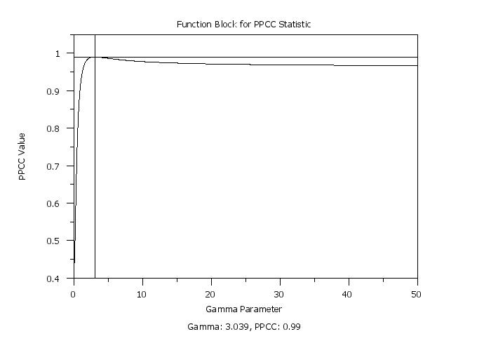
. Step 3:   Plot the function
.
title offset 2
title case asis
label case ais
y1tic mark offset 0  0.05
tic mark offset units data
y1label PPCC Value
x1label Gamma Parameter 
title Function Block for PPCC Statistic
plot f for gamma = 0.10 0.05 50
delete gamma
.
. Step 3:   Now use it to perform an optimization
.
let yopt = optimize f wrt gamma for gamma = 0.1 50
    

The following output is generated.

 MINIMUM OF A FUNCTION
       OPTIMIZATION VARIABLE             = GAMMA
       SPECIFIED LOWER LIMIT OF INTERVAL =         0.1000000000
       SPECIFIED UPPER LIMIT OF INTERVAL =        50.0000000000
  
       THE MINIMUM VALUE OCCURS AT =   0.3038950E+01
  
  
 THE COMPUTED VALUE OF THE CONSTANT   YOPT     =   0.3038950E+01
  
  
 THE COMPUTED VALUE OF THE CONSTANT   FVALUE   =  -0.9900165E+00
    

.
line dash
let fvalue = -fvalue
drawsdsd 15 fvalue 85 fvalue
drawdsds yopt 20 yopt 90
.
let gamma = round(yopt,3)
let ppcc = round(fvalue,3)
case asis
just center
move 50 5
text Gamma: ^gamma, PPCC: ^ppcc
    

 
. Purpose:  Demonstrate the use of function blocks in multivariate
.           optimization
.
. Step 1:   Read the data
.
skip 25
read weibbury.dat y
skip 0
.
. Step 2:   Define the function block
.
let n = size y
let ylog = log(y)
let ylogsum = sum ylog
let ylsd = sd ylog
let ghat = 1.28/ylsd
let ytemp = y**ghat
let sighat = sum ytemp
let sighat = sighat/n
.
capture function block one f a sigma gamma
let c1 = n*(log(gamma) - gamma*log(sigma))
let c2 = (gamma - 1)*ylogsum
let y2 = (y/sigma)**gamma
let c3 = sum y2
let a  = c1 + c2 - c3
end of capture
.
list function block one
    

The following output is generated.

.
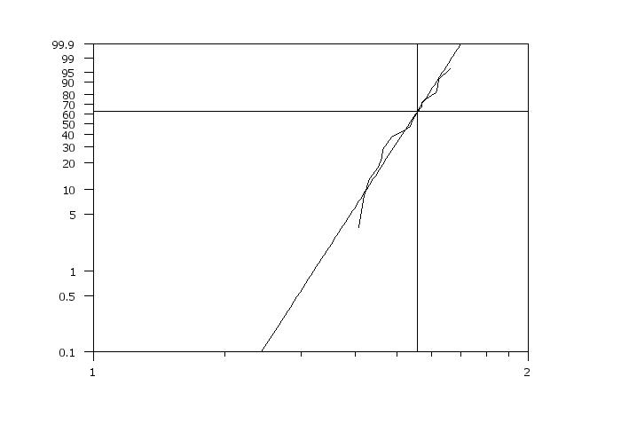
. Step 3:   Generate Weibull plot to obtain start values
.
weibull plot y
    



.
. Step 3:   Now use it to perform an optimization
.
let gamma = beta
let sigma = eta
set optimization maximum
optimization method line finite
let yopt = optimize f wrt sigma gamma
    

The following output is generated.

      MAXIMUM NUMBER OF ITERATIONS (  150) EXCEEDED.
  
       THE MINIMUM VALUE OCCURS AT = SIGMA       55.77204
       THE MINIMUM VALUE OCCURS AT = GAMMA       8.191590
    

.
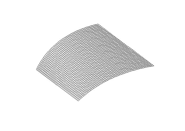
3d-plot f  for sigma = 40  0.5  60 for gamma = 5 0.1 10