EQUAL SLOPES TEST

EQUAL SLOPES TEST

Analysis Command

Test two or more linear regression lines to see if they have equal slopes.

It is occasionally of interest whether or not two regression lines have the same slope. That is, given
\( y_1 = a_1 + b_1 x_1 \)
\( y_2 = a_2 + b_2 x_2 \)

we want to test whether \( b_1 = b_2 \).

For example, this might be of interest when we are fitting a regression line based on two different measurement methods and we would like to know if the fits are equivalent.

If the residul variances from the two regressions are statistically equivalent, the test statstic is

\( \hat{t} = \frac{ |b_1 - b_2| } {\sqrt{c_1 c_2 }} \)

where

\( c_1 = \frac{s_{y_{1} \cdot x_{1}}^{2} (n_{1} - 2) + s_{y_{2} \cdot x_{2}}^{2} (n_{2} - 2)} {n_{1} + n_{2} - 4} \)

\( c_2 = \frac{1}{Q_{x_1}} + \frac{1} {Q_{x_2}} \)


\( s_{y \cdot x}^{2} = \frac{\sum{(y_{i} - \bar{y}}} {n - 2} \)

\( Q(x) = \sum{(x_{i} - \bar{x})^{2}} \)

This test statistic is compared to a t distribution with n₁ + n₂ - 4 degrees of freedom.

If the residual variances are not statistically equivalent and n₁ and n₂ are both greater than 20, the test statistic is

\( \hat{z} = \frac{|b_1 - b_2|} {\sqrt{\frac{s_{y_1 \cdot x_1}^{2}}{Q_{x_1}} \frac{s_{y_2 \cdot x_2}^{2}}{Q_{x_2}} }} \)

This is compared to a standard normal distribution. If n₁ or n₂ is less than or equal to 20, the test statistic is compared to a t distribution with ν degrees of freedom where

\( \nu = \frac{1}{\frac{c^2}{n_1 - 2} + \frac{(1 - c)^2}{n_2 - 2}} \)

\( c = \frac{\frac{s_{y_1 \cdot x_1}^{2}} {Q_{x_1}}} {\sqrt{ \frac{s_{y_1 \cdot x_1}^{2}} {Q_{x_1}} + \frac{s_{y_2 \cdot x_2}^{2}} {Q_{x_2}}} } \)

Note that n₁ should be set to the smaller sample size.

To determine whether the residual variances are equal, the test statistic is

\( \frac{s_{y_1 \cdot x_1}^{2}} {s_{y_1 \cdot x_1}^{2}} \)

The hypothesis of equal residual variances is rejected if this statistic is greater than the F percent point function with n₁ -2 and n₂ - 2 degrees of freedom.

Dataplot will perform the test for equal residual variances first and apply the appropriate test based on this.

For the case where three or more regression lines are being compared, a series of three tests are performed.

1. The first test is whether the k regressions are equal. The test statistic is
   \( F = \frac{\frac{1}{2k - 2} \left( Q_{y \cdot x; T} - \sum_{i=1}^{k}{Q_{y \cdot x; i}} \right) } {\frac{1}{n - 2k}\sum_{i=1}^{k}{Q_{y \cdot x; i}} } \)

   The hypothesis of equal regressions is rejected if this test statistic is greater than the F percent point function with 2k - 2 and n - 2k degrees of freedom.

   where

   \( Q_{y \cdot x} = \sum{(y_{i} - \hat{y})^{2}} \)

   That is, \( Q_{y \cdot x; T} \) is the sum of the squared differences between the data and the fitted function for the full data set while the \( Q_{y \cdot x; T} \) terms are the sum of the squared differences between the data and the fitted function for the k individual fits.

2. If the hypothesis of equal regressions is not rejected, nothing further is done. If the hypothesis is rejected, a test for equal slopes is performed. The test statistic is
   \( F = \frac{\frac{1}{k - 1} \left( A - \sum_{i=1}^{k}{Q_{y \cdot x; i}} \right) } {\frac{1}{n - 2k}\sum_{i=1}^{k}{Q_{y \cdot x; i}} } \)

   where

   \( A = \sum_{i=1}^{k}{Q_{y;i}} - \frac{\sum_{i=1}^{k}{Q_{xy;i}}} {\sum_{i=1}^{k}{Q_{x;i}}} \)

   \( Q_{xy} = \sum{(x - \bar{x}) (y - \bar{y})} \)

   The hypothesis of equal slopes is rejected if this test statistic is greater than the F percent point function with k - 1 and n - 2k degrees of freedom.

3. If the hypothesis of equal slopes is not rejected, nothing further is done. If the hypothesis is rejected, a test for equal intercepts is performed. The test statistic is
   \( F = \frac{\frac{1}{k - 1} \left( \sum_{i=1}^{k}{Q_{y \cdot x; T}} - A \right) } {\frac{1}{n - 2k}\sum_{i=1}^{k}{Q_{y \cdot x; i}} } \)

   The hypothesis of equal intercepts is rejected if this test statistic is greater than the F percent point function with k - 1 and n - 2k degrees of freedom.

EQUAL SLOPES TEST <y> <x> <tag>
                        <SUBSET/EXCEPT/FOR qualification>
where <y> is a response (= dependent) variable;
            <x> is a factor (= independent) variable;
            <tag> is a group-id variable;
and where the <SUBSET/EXCEPT/FOR qualification> is optional.

EQUAL SLOPE TEST Y X TAG
EQUAL SLOPE TEST Y X TAG SUBSET TAG 1 2 4 6

The following statistics are also supported
LET A = EQUAL SLOPES TEST Y X TAG
LET A = EQUAL SLOPES TEST CDF Y X TAG
LET A = EQUAL SLOPES TEST PVALUE Y X TAG
LET A = EQUAL SLOPES TEST CRITICAL VALUE Y X TAG


The critical value is the 95% critical value. For the more than two groups case, the values returned are the second of the three tests (i.e., the test for equal slopes).

In addition to the above LET command, built-in statistics are supported for 20+ different commands (enter HELP STATISTICS for details).

None

None

LINEAR CORRELATION PLOT	=	Generates a linear correlation plot.
LINEAR INTERCEPT PLOT	=	Generates a linear intercept plot.
LINEAR RESSD PLOT	=	Generates a linear residual standard deviation plot.
FIT	=	Carries out a least squares fit.

Lothar Sachs (1982), "Applied Statistics: A Handbook of Techniques", Springer-Verlag, pp. 413-442.

Exploratory Data Analysis

2015/10

 
. Step 1:   Read the data
.
dimension 40 columns
read y x indx
0.04101      297.16000        0.00000
0.04104      297.17000        0.00000
0.04105      297.18000        0.00000
0.04103      297.20000        0.00000
0.04109      297.20000        0.00000
0.03707      280.12000        0.00000
0.03929      290.12000        0.00000
0.04171      300.18000        0.00000
0.04428      310.18000        0.00000
0.04700      320.17000        0.00000
0.04052      297.15000        1.00000
0.04055      297.15000        1.00000
0.04056      297.15000        1.00000
0.04056      297.15000        1.00000
0.04056      297.15000        1.00000
0.03656      280.15000        1.00000
0.03883      290.15000        1.00000
0.04125      300.15000        1.00000
0.04381      310.15000        1.00000
0.04654      320.15000        1.00000
end of data
let n = size y
.
. Step 2:   Generate the individual fits
.
set write decimals 6
write "Fit for Lab One"
write " "
write " "
fit y x  subset indx = 0
let pred1 = pred
write " "
write " "
write "Fit for NIST"
write " "
write " "
fit y x  subset indx = 1
let pred2 = pred
.
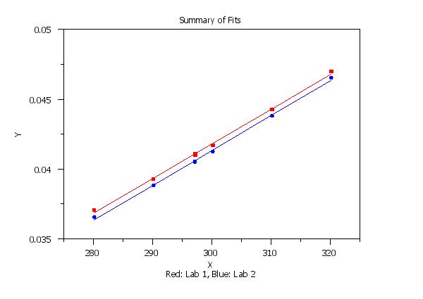
. Step 3:   Plot the fit
.
let x1 = x
let x2 = x
retain pred1 x1 subset indx = 0
retain pred2 x2 subset indx = 1
.
case asis
label case asis
title case asis
title offset 2
line blank blank solid solid
line color black black blue red
character circle box
character fill on on
character color blue red
char hw 1.0 0.75 all
y1label Y
x1label X
x2label Red: Lab 1, Blue: Lab 2
title Summary of Fits
.
ylimits 0.035 0.050
xlimits 280 320
xtic mark offset 5 5
.
plot y x subset indx = 1 and
plot y x subset indx = 0 and
plot pred2 x2 and
plot pred1 x1
.
. Step 4:   Perform the equal slopes test
.
let statva = equal slopes test y x indx
let statcd = equal slopes test cdf y x indx
let pval   = equal slopes test pvalue y x indx
let statcv = equal slopes test critical value y x indx
.
print statva statcd statcv pval
.
equal slopes test y x indx
    

The following output is generated

Fit for Lab One
 
 
  
             Least Squares Multilinear Fit
  
 Sample Size:                             10
 Number of Variables:                     1
 Residual Standard Deviation:             0.000122
 Residual Degrees of Freedom:             8
 BIC:                                     -177.777585
  
 Replication Case:
 Replication Standard Deviation:          0.000042
 Replication Degrees of Freedom:          1
 Number of Distinct Subsets:              9
 Lack of Fit F Ratio:                     9.381749
 Lack of Fit F CDF (%):                   75.360484
 Lack of Fit Degrees of Freedom 1:        7
 Lack of Fit Degrees of Freedom 2:        1
  
 --------------------------------------------------------------------
                                                Approximate
            Parameter Estimates          Standard Deviation   t-Value
 --------------------------------------------------------------------
   1  A0                      -0.032834            0.001143  -28.7237
   2  A1        X              0.000249            0.000004   65.0287
  
 
 
Fit for NIST
 
 
  
             Least Squares Multilinear Fit
  
 Sample Size:                             10
 Number of Variables:                     1
 Residual Standard Deviation:             0.000115
 Residual Degrees of Freedom:             8
 BIC:                                     -179.031014
  
 Replication Case:
 Replication Standard Deviation:          0.000017
 Replication Degrees of Freedom:          4
 Number of Distinct Subsets:              6
 Lack of Fit F Ratio:                     87.226813
 Lack of Fit F CDF (%):                   99.961750
 Lack of Fit Degrees of Freedom 1:        4
 Lack of Fit Degrees of Freedom 2:        4
  
 --------------------------------------------------------------------
                                                Approximate
            Parameter Estimates          Standard Deviation   t-Value
 --------------------------------------------------------------------
   1  A0                      -0.033728            0.001075  -31.3736
   2  A1        X              0.000250            0.000004   69.5272
 





 PARAMETERS AND CONSTANTS--

    STATVA  --      -0.265061
    STATCD  --       0.397174
    STATCV  --       2.119905
    PVAL    --       0.794347
  
             Summary Table
  
 -----------------------------------------------------------------
               Sample                                     Residual
   Group-ID      Size      Intercept          Slope       Variance
 -----------------------------------------------------------------
          1        10      -0.032834       0.000249       0.000000
          2        10      -0.033728       0.000250       0.000000
  
  
             Equal Slopes Test for Two Groups
             (Equal Residual Variances Case)
  
 Dependent (Y) Variable:  Y
 Independent (X) Variable:  X
 Group-ID Variable:   INDX
  
 H0: The Regression Slopes are Equal
 Ha: The Regression Slopes are not Equal
  
 Total Number of Observations:            20
 Number of Groups with Ni > 3:            2
  
 Test:
 Equal Slopes Test Statistic Value:       -0.265061
 CDF Value:                               0.397174
 P-Value:                                 0.794347
  
  
             Conclusions (Two-Tailed t-Test)
  
 H0: Slopes Are Equal
 ------------------------------------------------------------
                                                         Null
    Significance           Test       Critical     Hypothesis
           Level      Statistic   Region (+/-)     Conclusion
 ------------------------------------------------------------
           80.0%      -0.265061       1.336757         ACCEPT
           90.0%      -0.265061       1.745883         ACCEPT
           95.0%      -0.265061       2.119905         ACCEPT
           99.0%      -0.265061       2.920773         ACCEPT