
|
|
CONSENSUS MEAN PLOTName:
The CONSENSUS MEAN PLOT command performs a consensus means analysis and in addition to the textual output it presents the results in a graphical format. The details of the consensus means analysis are discussed in the documentation for the CONSENSUS MEANS command (enter HELP CONSENSUS MEANS for details). The graph consists of two parts. This plot allows you to compare the consensus values and associated uncertainties obtained by the different methods. It also allows you to compare the consensus values against the lab data. The methods are plotted in the following order:
In most cases, you will probably want only a subset of these methods. You can use the following commands to specify which methods to include in the consensus means analysis. This is demonstrated in the program samples below.
where <y> is the response variable; <tag> is the group-id variable; and where the <SUBSET/EXCEPT/FOR qualification> is optional. This is used for the raw data case.
<SUBSET/EXCEPT/FOR qualification> where <ymean> is the variable containing the lab means; <ysd> is the variable containing the lab standard deviations; <ni> is the variable containing the lab sample sizes; and where the <SUBSET/EXCEPT/FOR qualification> is optional. This is used for the summary data case.
<SUBSET/EXCEPT/FOR qualification> where <ymean> is the variable containing the lab means; <ysd> is the variable containing the lab standard deviations; <ni> is the variable containing the lab sample sizes; <labid> is the variable containing the lab-id's (numeric); and where the <SUBSET/EXCEPT/FOR qualification> is optional.
This is used for the summary data case. The
CONSENSUS MEAN PLOT Y TAG CONSENSUS MEAN PLOT Y TAG SUBSET TAG >= 2 CONSENSUS MEAN PLOT Y TAG SUBSET TAG = 1 TO 6 CONSENSUS MEAN PLOT YMEAN YSD NI
To reset the default of showing the lab data on the plot, enter
This is demonstrated in the Program 2 example below.
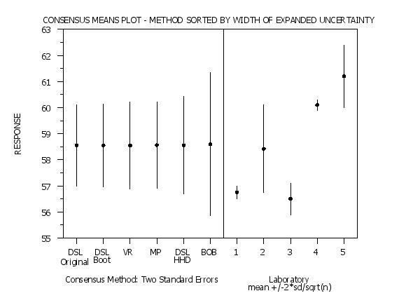
To reset the default of not sorting the methods, enter
This is demonstrated in the Program 3 example below. The program example shows how to read DPST3F.DAT to retrieve the sorted order of the methods.
In order to specify one or more labs to omit from the plot (but not the analysis), enter the command
where <lab1> ... <labk> is a list of 1 to 10 labs to be omitted from the plot. To reset the default of all labs being plotted, enter
This option was added 12/2016. Similarly, you can omit methods from the plot (but not the analysis) with the commands
SET CONSENSUS MEAN PLOT OMIT METHOD TWO <method> SET CONSENSUS MEAN PLOT OMIT METHOD THREE <method> When extreme outliers are included in the analysis, the results for some methods may distort the plot. This option was added 04/2017.
To reset the default, enter the commnd
This example is demonstrated in the Program 4 example below.
Graybill and Deal (1959), "Combining Unbiased Estimators", Biometrics, 15, pp. 543-550. M. S. Levenson, D. L. Banks, K. R. Eberhardt, L. M. Gill, W. F. Guthrie, H. K. Liu, M. G. Vangel, J. H. Yen, and N. F. Zhang (2000), "An ISO GUM Approach to Combining Results from Multiple Methods", Journal of Research of the National Institute of Standards and Technology, Volume 105, Number 4. John Mandel and Robert Paule (1970), "Interlaboratory Evaluation of a Material with Unequal Number of Replicates", Analytical Chemistry, 42, pp. 1194-1197. Robert Paule and John Mandel (1982), "Consensus Values and Weighting Factors", Journal of Research of the National Bureau of Standards, 87, pp. 377-385. Andrew Rukhin (2009), "Weighted Means Statistics in Interlaboratory Studies", Metrologia, Vol. 46, pp. 323-331. Andrew Ruhkin (2003), "Two Procedures of Meta-analysis in Clinical Trials and Interlaboratory Studies", Tatra Mountains Mathematical Publications, 26, pp. 155-168. Andrew Ruhkin and Mark Vangel (1998), "Estimation of a Common Mean and Weighted Means Statistics", Journal of the American Statistical Association, Vol. 93, No. 441. Andrew Ruhkin, B. Biggerstaff, and Mark Vangel (2000), "Restricted Maximum Likelihood Estimation of a Common Mean and Mandel-Paule Algorithm", Journal of Statistical Planning and Inference, 83, pp. 319-330. Mark Vangel and Andrew Ruhkin (1999), "Maximum Likelihood Analysis for Heteroscedastic One-Way Random Effects ANOVA in Interlaboratory Studies", Biometrics 55, 129-136. Susannah Schiller and Keith Eberhardt (1991), "Combining Data from Independent Analysis Methods", Spectrochimica, ACTA 46 (12). Susannah Schiller (1996), "Standard Reference Materials: Statistical Aspects of the Certification of Chemical SRMs", NIST SP 260-125, NIST, Gaithersburg, MD. Bimal Kumar Sinha (1985), "Unbiased Estimation of the Variance of the Graybill-Deal Estimator of the Common Mean of Several Normal Populations", The Canadian Journal of Statistics, Vol. 13, No. 3, pp. 243-247. Nien-Fan Zhang (2006), "The Uncertainty Associated with The Weighted Mean of Measurement Data", Metrologia, 43, PP. 195-204. Hagwood and Guthrie (2006), "Combining Data in Small Multiple-Methods Studies", Technometrics, Vol. 48, No. 2. Iyer, Wang, and Matthew (2004), "Models and Confidence Intervals for True Values in Interlaboratory Trials", Journal of the American Statistical Association, Vol. 99, No. 468, pp. 1060-1071. Fairweather (1972), "A Method for Obtaining an Exact Confidence Interval for the Common Mean of Several Normal Populations", Applied Statistics, Vol. 21, pp. 229-233. Cox (2002), "The Evaluation of Key Comparison Data", Metrologia, Vol. 39, pp. 589-595.
2011/10: Redesigned plot to incorporate the lab data 2016/12: Support for SET CONSENSUS MEAN PLOT OMIT LABS 2017/03: Support for SET CONSENSUS MEAN PLOT OMIT METHOD 2017/07: Changed the default for Schiller-Eberhardt, Fairweather, and Bayesian consensus procedure to OFF 2019/08: Added the command SET CONSENSUS MEAN PLOT DATA
. Step 1: Read the data
.
SKIP 25
READ STUTZ86.DAT ALITE JUNK2 JUNK3 JUNK4 JUNK5 LABID
.
. Step 2: Specify methods to include on the plot and define
.         strings containing method id's.  Define settings
.         for DerSimonian-Laird bootstrap.
.
set write decimals 5
set modified mandel paule off
set schiller eberhardt off
set mean of means off
set grand mean off
set graybill deal off
set generalized confidence interval off
set fairweather off
set bayesian consensus procedure off
set dersimonian laird minmax off
set dersimonian laird bootstrap on
.
let string sx1 = MP
let string sx2 = VR
let string sx3 = DSLcr()Original
let string sx4 = DSLcr()HHD
let string sx5 = DSLcr()Bootstrap
let string sx6 = BOB
let nmeth = 6
.
seed 21307
set random number generator fibonacci congruential
bootstrap samples 100000
.
. Step 3: Set plot control features
.
.         Settings for plot characters/lines
.
line solid all
character blank all
character fill on
character hw 1 0.75
character circle
line      blank
.
.         Settings for labels
.
case asis
title asis
title offset 2
tic mark label case asis
title Consensus Means Plot
y1label Response
.
let nlab = unique labid
loop for k = 1 1 nlab
     let icnt = k + nmeth
     let string sx^icnt = ^k
end of loop
.
let ntot = nmeth + nlab
xlimits 1 ntot
major xtic mark number ntot
minor xtic mark number 0
tic mark offset units data
xtic mark offset 0.5   0.5
x1tic mark label format group label
let igx = group label sx1 to sx^ntot
x1tic mark label content igx
.
. Step 4: Generate the plot
.
set consensus mean plot error two standard errors
feedback off
consensus mean plot alite labid
.
. Step 5: Post plot labelling
.
line dotted
drawdsds  6.5 20  6.5 90
justification center
moveds 3.5 5
text Consensus Method: Two Standard Errors
moveds 9 5
text Laboratorycr()meansp()+/-2*sd/sqrt(n)
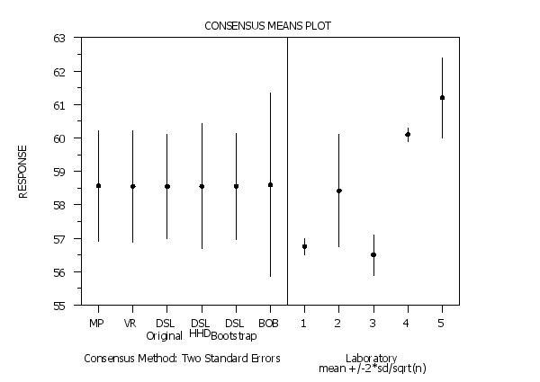 Program 2:
. This version suppresses the lab data portion of the plot
.
. Step 1: Read the data
.
SKIP 25
READ STUTZ86.DAT ALITE JUNK2 JUNK3 JUNK4 JUNK5 LABID
.
. Step 2: Specify methods to include on the plot and define
.         strings containing method id's.  Define settings
.         for DerSimonian-Laird bootstrap.
.
set write decimals 5
set modified mandel paule off
set schiller eberhardt off
set mean of means off
set grand mean off
set graybill deal off
set generalized confidence interval off
set fairweather off
set bayesian consensus procedure off
set dersimonian laird minmax off
set dersimonian laird bootstrap on
.
let string sx1 = MP
let string sx2 = VR
let string sx3 = DSLcr()Original
let string sx4 = DSLcr()HHD
let string sx5 = DSLcr()Bootstrap
let string sx6 = BOB
let nmeth = 6
.
seed 21307
set random number generator fibonacci congruential
bootstrap samples 100000
.
. Step 3: Set plot control features
.
.         Settings for plot characters/lines
.
line solid all
character blank all
character fill on
character hw 1 0.75
character circle
line      blank
.
.         Settings for labels
.
case asis
title asis
title offset 2
tic mark label case asis
title Consensus Means Plot
y1label Response
.
xlimits 1 nmeth
major xtic mark number nmeth
minor xtic mark number 0
tic mark offset units data
xtic mark offset 0.5   0.5
x1tic mark label format group label
let igx = group label sx1 to sx^nmeth
x1tic mark label content igx
x1label Consensus Method: Two Standard Errors
x1label displacement 15
.
title Consensus Means Plot - Lab Data Omitted
set consensus mean plot data off
feedback off
consensus mean plot alite labid
 Program 3:
. Step 1: Read the data
.
SKIP 25
READ STUTZ86.DAT ALITE JUNK2 JUNK3 JUNK4 JUNK5 LABID
.
. Step 2: Specify methods to include on the plot and define
.         strings containing method id's.  Define settings
.         for DerSimonian-Laird bootstrap.
.
set write decimals 5
set modified mandel paule off
set schiller eberhardt off
set mean of means off
set grand mean off
set graybill deal off
set generalized confidence interval off
set fairweather off
set bayesian consensus procedure off
set dersimonian laird minmax off
set dersimonian laird bootstrap on
.
let string sx1 = MP
let string sx2 = VR
let string sx3 = DSLcr()Original
let string sx4 = DSLcr()HHD
let string sx5 = DSLcr()Boot
let string sx6 = BOB
let nmeth = 6
.
seed 21307
set random number generator fibonacci congruential
bootstrap samples 100000
.
. Step 3: Set plot control features
.
.         Settings for plot characters/lines
.
line solid all
character blank all
character fill on
character hw 1 0.75
character circle
line      blank
.
.         Settings for labels
.
case asis
title asis
title offset 2
tic mark label case asis
y1label Response
.
let nlab = unique labid
loop for k = 1 1 nlab
     let icnt = k + nmeth
     let string sx^icnt = ^k
end of loop
.
let ntot = nmeth + nlab
xlimits 1 ntot
major xtic mark number ntot
minor xtic mark number 0
tic mark offset units data
xtic mark offset 0.5   0.5
x1tic mark label format group label
let igx = group label sx1 to sx^ntot
x1tic mark label content igx
.
. Step 4: Generate the plot
.
loop for k = 1 1 ntot
    let string sxnew^k = ^sx^k
end of loop
.
.         Generate dummy plot, read dpst3f.dat to obtain
.         sorted labels
.
set consensus mean plot sorted on
set consensus mean plot error two standard errors
.
device 1 off
device 2 off
print off
consensus mean plot alite labid
skip 0
read dpst3f.dat indx
loop for k = 1 1 nmeth
    let icnt = indx(k)
    let string sxnew^k = ^sx^icnt
end of loop
let igx = group label sxnew1 to sxnew^ntot
x1tic mark label content igx
device 1 on
device 2 on
printing on
.
.         Now generate plot with sorted labels
.
title Consensus Means Plot - Method Sorted by Width of Expanded Uncertainty
feedback off
consensus mean plot alite labid
.
. Step 5: Post plot labelling
.
line dotted
drawdsds  6.5 20  6.5 90
justification center
moveds 3.5 5
text Consensus Method: Two Standard Errors
moveds 9 5
text Laboratorycr()meansp()+/-2*sd/sqrt(n)
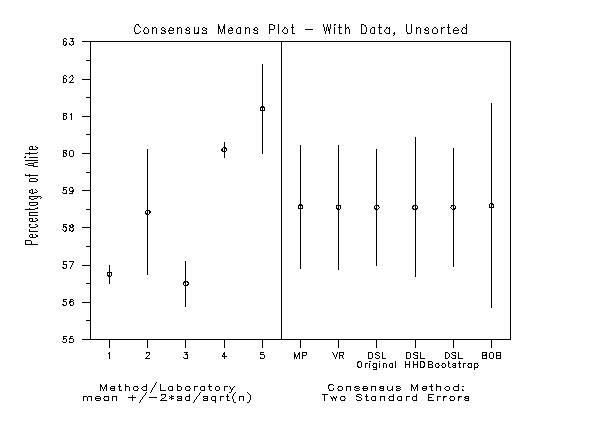
 Program 4:
. Step 1:   Read the data
.
SKIP 25
READ STUTZ86.DAT ALITE JUNK2 JUNK3 JUNK4 JUNK5 LABID
.
. Step 2:   Define consensus means options
.
set write decimals 5
set bob on
set dersimonian laird bootstrap on
set dersimonian laird minmax off
set modified mandel paule off
set schiller eberhardt off
set mean of means off
set grand mean off
set graybill deal off
set generalized confidence interval off
set fairweather off
set bayesian consensus procedure off
set random number generator fibonacci congruential
seed 55631
bootstrap samples 100000
.
.  iflagm  = 1   => 95% Confidence Interval
.          = 2   => Two Standard Errors Confidence Interval
.          = 3   => One Standard Errors Confidence Interval
.
let iflagm = 2
if iflagm = 1
   set consensus mean plot error confidence intervals
else if iflagm = 2
   set consensus mean plot error two standard errors
else if iflagm = 3
   set consensus mean plot error one standard errors
end of if
.
.
. Step 3:   Define strings containing Method id's
.
let nlab = unique labid
loop for k = 1 1 nlab
     let string sx^k = ^k
end of loop
.
let icnt = nlab + 1
let string sx^icnt = MP
let icnt = icnt + 1
let string sx^icnt = VR
let icnt = icnt + 1
let string sx^icnt = DSLcr()Original
let icnt = icnt + 1
let string sx^icnt = DSLcr()HHD
let icnt = icnt + 1
let string sx^icnt = DSLcr()Bootstrap
let icnt = icnt + 1
let string sx^icnt = BOB
let nmeth = 6
.
. Step 4:   Set plot control options
.
line solid all
character blank all
character fill on
character hw 1 0.75
character circle
line      blank
.
case asis
title case asis
label case asis
tic mark label case asis
title offset 2
title Consensus Means Plot - With Data, Unsorted
y1label Percentage of Alite
.
let ntot = nmeth + nlab
xlimits 1 ntot
major xtic mark number ntot
minor xtic mark number 0
tic mark offset units data
xtic mark offset 0.5   0.5
x1tic mark label format group label
let igx = group label sx1 to sx^ntot
x1tic mark label content igx
.
. Step 5:   Generate the consensus mean plot
.
set consensus mean plot data left
. printing off
capture screen on
capture cmplot.out
consensus mean plot alite labid
end of capture
. printing on
.
line dotted
drawdsds  5.5 20  5.5 90
.
justification center
moveds 8.5 8
if iflagm = 1
   text Consensus Method:cr()95% Confidence Limits
else if iflagm = 2
   text Consensus Method:cr()Two Standard Errors
else if iflagm = 3
   text Consensus Method:cr()One Standard Error
end of if
moveds 2.5 8
text Method/Laboratorycr()meansp()+/-2*sd/sqrt(n)
Date created: 08/17/2001 |
Last updated: 12/04/2023 Please email comments on this WWW page to [email protected]. | ||||||||||||||||||||||||||||||||||||||||||||||||||