|
Global Prediction
|
How does one predict the response at points other than those
used in the experiment? The prediction equation yields good
results at the eight combinations of coded -1 and +1 values for
the three factors:
- X1 = Number of turns = 90 and 180
- X2 = Winding distance = 0.38 and 1.14
- X3 = Wire gauge = 40 and 48
What, however, would one expect the detector to yield at target
settings of, say,
- Number of turns = 150
- Winding distance = 0.50
- Wire gauge = 46
Based on the fitted equation, we first translate the target values
into coded target values as follows:
coded target = -1 + 2*(target-low)/(high-low)
Hence the coded target values are
- X1 = -1 + 2*(150-90)/(180-90) = 0.333333
- X2 = -1 + 2*(0.50-0.38)/(1.14-0.38) = -0.684211
- X3 = -1 + 2*(46-40)/(48-40) = 0.5000
Thus the raw data
(Number of turns, Winding distance, Wire gauge) = (150, 0.50, 46)
translates into the coded
(X1, X2, X3) = (0.333333, -0.684211, 0.50000)
on the -1 to +1 scale.
Inserting these coded values into the fitted equation yields,
as desired, a predicted value of
\( \hat{Y} \)
= 2.65875 + 1.55125(0.333333) - 0.43375(-0.684211)
= 3.47261
The above procedure can be carried out for any values of turns,
distance, and gauge. This is subject to the usual cautions that
equations that are good near the data point vertices may not
necessarily be good everywhere in the factor space. Interpolation is a
bit safer than extrapolation, but it is not guaranteed to provide
good results, of course.
One would feel more comfortable about interpolation (as in our
example) if additional data had been collected at the center
point and the center point data turned out to be in good agreement
with predicted values at the center point based on the fitted
model. In our case, we had no such data and so the sobering
truth is that the user of the equation is assuming something in
which the data set as given is not capable of suggesting one way or
the other. Given that assumption, we have demonstrated how one
may cautiously but insightfully generate predicted values that
go well beyond our limited original data set of eight points.
|
|
Global Determination of Best Settings
|
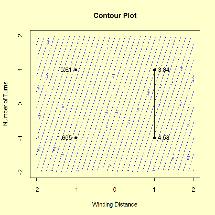
In order to determine the best settings for the factors, we can
use a
DOE contour plot.
The DOE contour plot is generated for the two most significant
factors and shows the value of the response variable at the
vertices (i.e, the -1 and +1 settings for the factor variables)
and indicates the direction that maximizes (or minimizes) the
response variable. If you have more than
two significant factors, you can generate a series of DOE
contour plots with each one using two of the important factors.
|


