5.6. Case Studies
5.6.1. Eddy Current Probe Sensitivity Case Study
5.6.1.9. |
Validate the Fitted Model |
-
\( \hat{Y} = 2.65875 + 1.55125 X_{1} - 0.43375 X_{2} \)
The next step is to validate the model. The primary method of model validation is graphical residual analysis; that is, through an assortment of plots of the differences between the observed data Y and the predicted value \( \scriptsize \hat{Y} \) from the model. For example, the design point (-1, -1, -1) has an observed data point (from the Background and data section) of Y = 1.70, while the predicted value from the above fitted model for this design point is
-
\( \hat{Y} = 2.65875 + 1.55125 (-1) - 0.43375 (-1) \)
   X1   X2   X3  Observed Predicted  Residual
----------------------------------------------
   -1   -1   -1    1.70    1.54125    0.15875
   +1   -1   -1    4.57    4.64375   -0.07375
   -1   +1   -1    0.55    0.67375   -0.12375
   +1   +1   -1    3.39    3.77625   -0.38625
   -1   -1   +1    1.51    1.54125   -0.03125
   +1   -1   +1    4.59    4.64375   -0.05375
   -1   +1   +1    0.67    0.67375   -0.00375
   +1   +1   +1    4.29    3.77625    0.51375
-
\( s_{res} = \sqrt{ \frac{\sum_{i=1}^{N}{r_{i}^{2}}} {N-P}} \)
Further, if the model is adequate and complete, the residuals should have no structural relationship with any other variables that may have been recorded. In particular, this includes the run sequence (time), which is really serving as a surrogate for any physical or environmental variable correlated with time. Ideally, all such residual scatter plots should appear structureless. Any scatter plot that exhibits structure suggests that the factor should have been formally included as part of the prediction equation.
Validating the prediction equation thus means that we do a final check as to whether any other variables may have been inadvertently left out of the prediction equation, including variables drifting with time.
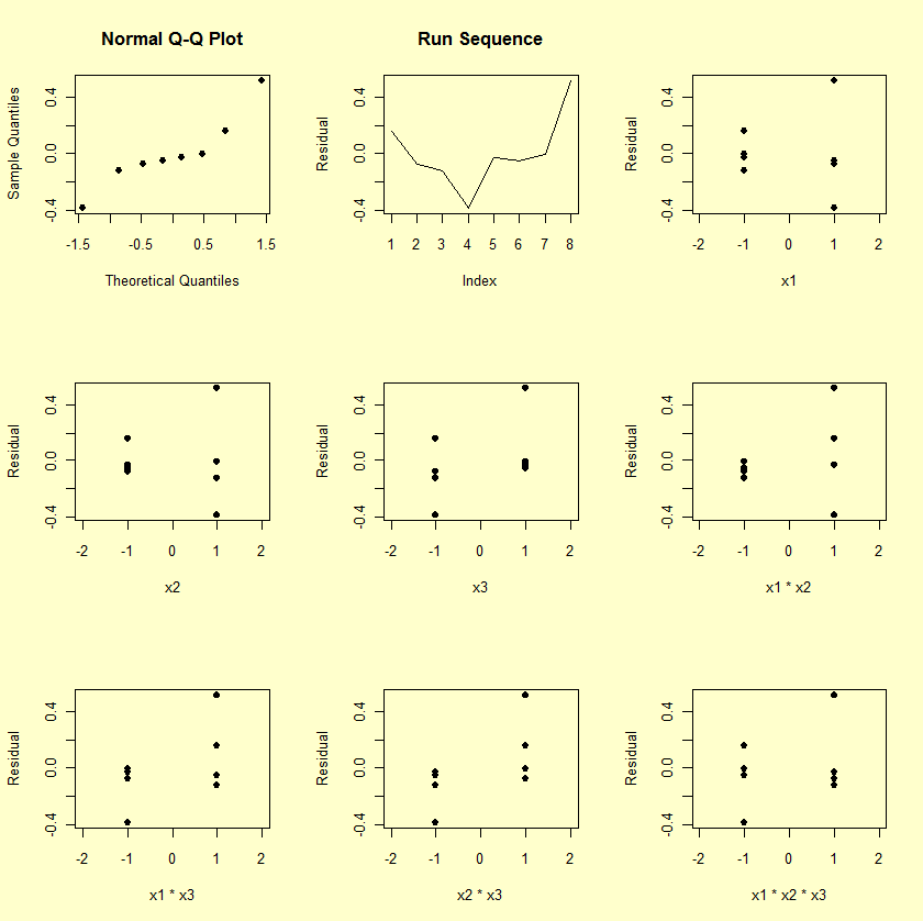
The graphical residual analysis thus consists of scatter plots of the residuals versus all three factors and four interactions (all such plots should be structureless), a scatter plot of the residuals versus run sequence (which also should be structureless), and a normal probability plot of the residuals (which should be near linear). We present such plots below.
The first plot is a normal probability plot of the residuals. The second plot is a run sequence plot of the residuals. The remaining plots show the residuals plotted against each of the factors and each of the interaction terms.
- Main Effects and Interactions: The X1 and X2 scatter
plots are "flat" (as they must be since
X1 and X2
were explicitly included in the model). The X3 plot shows
some structure as does the X1*X3, the
X2*X3, and the
X1*X2*X3 plots.
The X1*X2 plot shows little structure. The net
effect is that the relative ordering of these scatter plots is
very much in agreement (again, as it must be) with the relative
ordering of the "unimportant" factors.
From the table of effects
and the X2*X3 residual plot, the
third most influential term to be added to the model would
be X2*X3. In effect, these plots offer a
higher-resolution confirmation of the ordering of effects.
On the other hand, none of these other factors "passed" the
criteria given in the previous section, and so these
factors, suggestively influential as they might be, are
still not influential enough to be added to the model.
- Time Drift: The run sequence scatter plot is random. Hence
there does not appear to be a drift either from time, or from
any factor (e.g., temperature, humidity, pressure, etc.)
possibly correlated with time.
- Normality: The normal probability plot of the eight residuals has some trend, which suggests that additional terms might be added. On the other hand, the correlation coefficient of the 8 ordered residuals and the eight theoretical normal N(0,1) order statistic medians (which define the two axes of the plot) has the value 0.934, which is well within acceptable (5 %) limits of the normal probability plot correlation coefficient test for normality. Thus, the plot is not so non-linear as to reject normality.
-
\( \hat{Y} = 2.65875 + 1.55125 X_{1} - 0.43375 X_{2} \)


