5. Process Improvement
5.5. Advanced topics
5.5.9. An EDA approach to experimental design
5.5.9.10. DOE contour plot

5.5.9.10.7.

How to Interpret: Optimal Setting

Optimal setting

The "near-point" optimality setting is the intersection of the steepest-ascent line with the optimal setting curve.

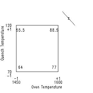
Theoretically, any (X₁, X₃) setting along the optimal curve would generate the desired response of Y = 100. In practice, however, this is true only if our estimated contour surface is identical to "nature's" response surface. In reality, the plotted contour curves are truth estimates based on the available (and "noisy") n = 8 data values. We are confident of the contour curves in the vicinity of the data points (the four corner points on the chart), but as we move away from the corner points, our confidence in the contour curves decreases. Thus the point on the Y = 100 optimal response curve that is "most likely" to be valid is the one that is closest to a corner point. Our objective then is to locate that "near-point".

Defective springs example

In terms of the defective springs contour plot, we draw a line from the best corner, (+, +), outward and perpendicular to the Y = 90, Y = 95, and Y = 100 contour curves. The Y = 100 intersection yields the "nearest point" on the optimal response curve.

Having done so, it is of interest to note the coordinates of that optimal setting. In this case, from the graph, that setting is (in coded units) approximately at

(X₁ = 1.5, X₃ = 1.3)

Table of coded and uncoded factors

With the determination of this setting, we have thus, in theory, formally completed our original task. In practice, however, more needs to be done. We need to know "What is this optimal setting, not just in the coded units, but also in the original (uncoded) units"? That is, what does (X₁=1.5, X₃=1.3) correspond to in the units of the original data?

To deduce his, we need to refer back to the original (uncoded) factors in this problem. They were:

Coded Factor	Uncoded Factor
X1	OT: Oven Temperature
X2	CC: Carbon Concentration
X3	QT: Quench Temperature

Uncoded and coded factor settings

These factors had settings-- what were the settings of the coded and uncoded factors? From the original description of the problem, the uncoded factor settings were:

1. Oven Temperature (1450 and 1600 degrees)
2. Carbon Concentration (0.5 % and 0.7 %)
3. Quench Temperature (70 and 120 degrees)

with the usual settings for the corresponding coded factors:

1. X₁ (-1, +1)
2. X₂ (-1, +1)
3. X₃ (-1, +1)

Diagram

To determine the corresponding setting for (X₁=1.5, X₃=1.3), we thus refer to the following diagram, which mimics a scatter plot of response averages--oven temperature (OT) on the horizontal axis and quench temperature (QT) on the vertical axis:

The "X" on the chart represents the "near point" setting on the optimal curve.

Optimal setting for X₁ (oven temperature)

To determine what "X" is in uncoded units, we note (from the graph) that a linear transformation between OT and X₁ as defined by

OT = 1450 => X₁ = -1
OT = 1600 => X₁ = +1

yields

X₁ = 0 being at OT = (1450 + 1600) / 2 = 1525

thus

           |-------------|-------------|
X1:       -1             0            +1
OT:      1450          1525          1600

and so X₁ = +2, say, would be at oven temperature OT = 1675:

           |-------------|-------------|-------------|
X1:       -1             0            +1            +2
OT:      1450          1525          1600          1675

and hence the optimal X₁ setting of 1.5 must be at

OT = 1600 + 0.5*(1675-1600) = 1637.5

Optimal setting for X₃ (quench temperature)

Similarly, from the graph we note that a linear transformation between quench temperature QT and coded factor X₃ as specified by

QT = 70 => X₃ = -1
QT = 120 => X₃ = +1

yields

X₃ = 0 being at QT = (70 + 120) / 2 = 95

as in

        |-------------|-------------|
X3:    -1             0            +1
QT:    70            95           120

and so X₃ = +2, say, would be quench temperature = 145:

        |-------------|-------------|-------------|
X3:    -1             0            +1            +2
QT:    70            95           120           145

Hence, the optimal X₃ setting of 1.3 must be at

QT = 120 + 0.3*(145-120)
QT = 127.5

Summary of optimal settings

In summary, the optimal setting is

coded : (X₁ = +1.5, X₃ = +1.3)
uncoded: (OT = 1637.5 degrees, QT = 127.5 degrees)

and finally, including the best setting of the fixed X₂ factor (carbon concentration CC) of X₂ = -1 (CC = 0.5 %), we thus have the final, complete recommended optimal settings for all three factors:

coded : (X₁ = +1.5, X₂ = -1.0, X₃ = +1.3)
uncoded: (OT = 1637.5, CC = 0.7 %, QT = 127.5)

If we were to run another experiment, this is the point (based on the data) that we would set oven temperature, carbon concentration, and quench temperature with the hope/goal of achieving 100 % acceptable springs.

Options for next step

In practice, we could either

1. collect a single data point (if money and time are an issue) at this recommended setting and see how close to 100 % we achieve, or

2. collect two, or preferably three, (if money and time are less of an issue) replicates at the center point (recommended setting).

3. if money and time are not an issue, run a 2² full factorial design with center point. The design is centered on the optimal setting (X₁ = +1, 5, X₃ = +1.3) with one overlapping new corner point at (X₁ = +1, X₃ = +1) and with new corner points at (X₁, X₃) = (+1, +1), (+2, +1), (+1, +1.6), (+2, +1.6). Of these four new corner points, the point (+1, +1) has the advantage that it overlaps with a corner point of the original design.