5. Process Improvement
5.5. Advanced topics
5.5.9. An EDA approach to experimental design
5.5.9.9. Cumulative residual standard deviation plot

5.5.9.9.10.

Motivation: How do we Use the Model for Interpolation?

Design table in original data units

As for the mechanics of interpolation itself, consider a continuation of the prior k = 2 factor experiment. Suppose temperature T ranges from 300 to 350 and time t ranges from 20 to 30, and the analyst can afford n = 4 runs. A 2² full factorial design is run. Forming the coded temperature as X₁ and the coded time as X₂, we have the usual:

Temperature	Time	X1	X2	Y
300	20	-	-	2
350	20	+	-	4
300	30	-	+	6
350	30	+	+	8

Graphical representation

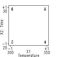
Graphically the design and data are as follows:

Typical interpolation question

As before, from the data, the prediction equation is

\( \hat{Y} = 5 + 2 X_{2} + X_{1} \)

We now pose the following typical interpolation question:

From the model, what is the predicted response at, say, temperature = 310 and time = 26?

In short:

\( \hat{Y}(T = 310, t = 26) = \mbox{?} \)

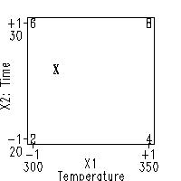
To solve this problem, we first view the k = 2 design and data graphically, and note (via an "X") as to where the desired (T = 310, t = 26) interpolation point is:

Predicting the response for the interpolated point

The important next step is to convert the raw (in units of the original factors T and t) interpolation point into a coded (in units of X₁ and X₂) interpolation point. From the graph or otherwise, we note that a linear translation between T and X₁, and between t and X₂ yields

T = 300 => X₁ = -1
T = 350 => X₁ = +1

thus

X₁ = 0 is at T = 325

        |-------------|-------------|
       -1     ?       0            +1
       300   310     325           350
   

which in turn implies that

T = 310 => X₁ = -0.6

Similarly,

t = 20 => X₂ = -1
t = 30 => X₂ = +1

therefore,

X₂ = 0 is at t = 25

        |-------------|-------------|
       -1             0   ?        +1
       20             25 26        30
   

thus

t = 26 => X₂ = +0.2

Substituting X₁ = -0.6 and X₂ = +0.2 into the prediction equation

\( \hat{Y} = 5 + 2 X_{2} + X_{1} \)

yields a predicted value of 4.8.

Graphical representation of response value for interpolated data point

Thus