5. Process Improvement
5.5. Advanced topics
5.5.3. How do you optimize a process?
5.5.3.1. Single response case

5.5.3.1.1.

Single response: Path of steepest ascent

Starting at the current operating conditions, fit a linear model

If experimentation is initially performed in a new, poorly understood production process, chances are that the initial operating conditions X₁, X₂, ...,X_k are located far from the region where the factors achieve a maximum or minimum for the response of interest, Y. A first-order model will serve as a good local approximation in a small region close to the initial operating conditions and far from where the process exhibits curvature. Therefore, it makes sense to fit a simple first-order (or linear polynomial) model of the form:

\( \hat{Y} = \beta_{0} + \beta_{1} X_{1} + \beta_{2} X_{2} + \cdots + \beta_{k} X_{k} \)

Experimental strategies for fitting this type of model were discussed earlier. Usually, a 2^k-p fractional factorial experiment is conducted with repeated runs at the current operating conditions (which serve as the origin of coordinates in orthogonally coded factors).

Determine the directions of steepest ascent and continue experimenting until no further improvement occurs - then iterate the process

The idea behind "Phase I" is to keep experimenting along the direction of steepest ascent (or descent, as required) until there is no further improvement in the response. At that point, a new fractional factorial experiment with center runs is conducted to determine a new search direction. This process is repeated until at some point significant curvature in \( \hat{Y} \) is detected. This implies that the operating conditions X₁, X₂, ...,X_k are close to where the maximum (or minimum, as required) of Y occurs. When significant curvature, or lack of fit, is detected, the experimenter should proceed with "Phase II". Figure 5.2 illustrates a sequence of line searches when seeking a region where curvature exists in a problem with 2 factors (i.e., k=2).

FIGURE 5.2: A Sequence of Line Searches for a 2-Factor Optimization Problem

Two main decisions: search direction and length of step

There are two main decisions an engineer must make in Phase I:

1. determine the search direction;
2. determine the length of the step to move from the current operating conditions.

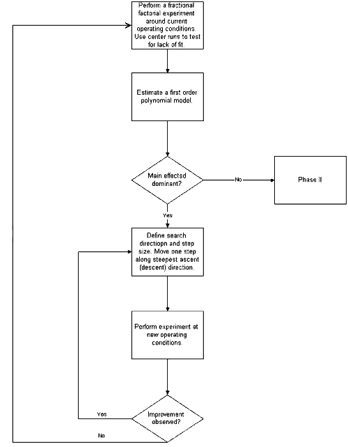
Figure 5.3 shows a flow diagram of the different iterative tasks required in Phase I. This diagram is intended as a guideline and should not be automated in such a way that the experimenter has no input in the optimization process.

Flow chart of iterative search process

FIGURE 5.3: Flow Chart for the First Phase of the Experimental Optimization Procedure

Procedure for Finding the Direction of Maximum Improvement

The direction of steepest ascent is determined by the gradient of the fitted model

Suppose a first-order model (like above) has been fit and provides a useful approximation. As long as lack of fit (due to pure quadratic curvature and interactions) is very small compared to the main effects, steepest ascent can be attempted. To determine the direction of maximum improvement we use

1. the estimated direction of steepest ascent, given by the gradient of \( \hat{Y} \), if the objective is to maximize Y;
2. the estimated direction of steepest descent, given by the negative of the gradient of \hat{Y} \), if the objective is to minimize Y.

The direction of steepest ascent depends on the scaling convention - equal variance scaling is recommended

The direction of the gradient, g, is given by the values of the parameter estimates, that is, g' = (b₁, b₂, ..., b_k). Since the parameter estimates b₁, b₂, ..., b_k depend on the scaling convention for the factors, the steepest ascent (descent) direction is also scale dependent. That is, two experimenters using different scaling conventions will follow different paths for process improvement. This does not diminish the general validity of the method since the region of the search, as given by the signs of the parameter estimates, does not change with scale. An equal variance scaling convention, however, is recommended. The coded factors x_i, in terms of the factors in the original units of measurement, X_i, are obtained from the relation

\( x_{i} = \frac{X_{i} - \left( X_{\mbox{low}} + X_{\mbox{high}} \right)/2} {\left( X_{\mbox{high}} - X_{\mbox{low}} \right)/2} \hspace{.5in} i = 1, 2, \dots , k \)

This coding convention is recommended since it provides parameter estimates that are scale independent, generally leading to a more reliable search direction. The coordinates of the factor settings in the direction of steepest ascent, positioned a distance \( \rho \) from the origin, are given by:

\( \mbox{maximize} \hspace{.3in} \beta_{0} + \beta_{1}x_{1} + \beta_{2}x_{2} + \cdots + \beta_{k}x_{k} \)

\( \mbox{subject to:} \hspace{.2in} \sum_{i=1}^{k}{x_{i}^{2}} \le \rho^{2} \)

Solution is a simple equation

This problem can be solved with the aid of an optimization solver (e.g., like the solver option of a spreadsheet). However, in this case this is not really needed, as the solution is a simple equation that yields the coordinates

\( x_{i}^{*} = \rho \frac{\beta_{i}} {\sqrt{\sum_{j=1}^{k}{\beta_{j}^{2}}}} \hspace{.5in} i = 1, 2, \ldots , k \).

Equation can be computed for increasing values of

An engineer can compute this equation for different increasing values of \( \rho \) and obtain different factor settings, all on the steepest ascent direction.

To see the details that explain this equation, see Technical Appendix 5A.

Example: Optimization of a Chemical Process

Optimization by search example

It has been concluded (perhaps after a factor screening experiment) that the yield (Y, in %) of a chemical process is mainly affected by the temperature (X₁, in C) and by the reaction time (X₂, in minutes). Due to safety reasons, the region of operation is limited to

  50 ≤ X₁ ≤ 250
150 ≤ X₂ ≤ 500

Factor levels

The process is currently run at a temperature of 200 \( ^{\circ} \mbox{C} \) and a reaction time of 200 minutes. A process engineer decides to run a 2² full factorial experiment with factor levels at

factor	low	center	high
X1	170	200	230
X2	150	200	250

Orthogonally coded factors

Five repeated runs at the center levels are conducted to assess lack of fit. The orthogonally coded factors are

\( x_{1} = \frac{X_{1} - 200}{30} \hspace{.3in}\) and \( \hspace{.3in} x_{2} = \frac{X_{2} - 200}{50} \).

Experimental results

The experimental results were:

x1	x2	X1	X2	Y (= yield)
-1	-1	170	150	32.79
+1	-1	230	150	24.07
-1	+1	170	250	48.94
+1	+1	230	250	52.49
0	0	200	200	38.89
0	0	200	200	48.29
0	0	200	200	29.68
0	0	200	200	46.50
0	0	200	200	44.15

(The reader can download the data as a text file.)

ANOVA table

The corresponding ANOVA table for a first-order polynomial model is

                 SUM OF        MEAN    F
SOURCE          SQUARES   DF  SQUARE  VALUE  PROB>F
MODEL          503.3035   2  251.6517 4.7972 0.0687
CURVATURE        8.2733   1    8.2733 0.1577 0.7077
RESIDUAL       262.2893   5   52.4579
  LACK OF FIT   37.6382   1   37.6382 0.6702 0.4590
  PURE ERROR   224.6511   4   56.1628

COR TOTAL      773.8660   8

Resulting model

It can be seen from the ANOVA table that there is no significant lack of linear fit due to an interaction term and there is no evidence of curvature. Furthermore, there is evidence that the first-order model is significant. The resulting model (in the coded variables) is

\( \hat{Y} = 40.644 - 1.2925 x_{1} + 11.14 x_{2} \)

Diagnostic checks

The usual diagnostic checks show conformance to the regression assumptions, although the R² value is not very high: R² = 0.6504.

Determine level of factors for next run using direction of steepest ascent

To maximize \( \hat{Y} \), we use the direction of steepest ascent. The engineer selects \( \rho \) = 1 since a point on the steepest ascent direction one unit (in the coded units) from the origin is desired. Then from the equation above for the predicted Y response, the coordinates of the factor levels for the next run are given by:

\( \begin{array}{lcl} x_{1}^{*} & = & \frac{\rho \beta_{1}}{\sqrt{\sum_{j=1}^{2}{\beta_{j}^{2}}}} \\ & = & \frac{(1)(-1.2925)}{\sqrt{(-1.2925)^{2} + (11.14)^2}} \\ & = & -0.1152 \end{array} \)

and

\( \begin{array}{lcl} x_{2}^{*} & = & \frac{\rho \beta_{2}}{\sqrt{\sum_{j=1}^{2}{\beta_{j}^{2}}}} \\ & = & \frac{(1)(11.14)}{\sqrt{(-1.2925)^{2} + (11.14)^2}} \\ & = & 0.9933 \end{array} \)

This means that to improve the process, for every (-0.1152)(30) = -3.456 \( ^{\circ} C \) that temperature is varied (decreased), the reaction time should be varied by (0.9933)(50) = 49.66 minutes.

---

Technical Appendix 5A: finding the factor settings on the steepest ascent direction a specified distance from the origin

Details of how to determine the path of steepest ascent

The problem of finding the factor settings on the steepest ascent/descent direction that are located a distance \( \rho \) from the origin is given by the optimization problem,

\( \mbox{maximize} \hspace{.3in} \beta_{0} + \beta_{1}x_{1} + \beta_{2}x_{2} + \cdots + \beta_{k}x_{k} \)
\( \mbox{subject to:} \hspace{.2in} \sum_{i=1}^{k}{x_{i}^{2}} \le \rho^{2} \)

Solve using a Lagrange multiplier approach

To solve it, use a Lagrange multiplier approach. First, add a penalty \( \lambda \) for solutions not satisfying the constraint (since we want a direction of steepest ascent, we maximize, and therefore the penalty is negative). For steepest descent we minimize and the penalty term is added instead.

\( \mbox{maximize} \hspace{.3in} L = b'x - \lambda(x'x - \rho^{2}) \)

Compute the partials and equate them to zero

\( \frac{\partial L}{\partial x} = b - 2 \lambda x = 0 \)

\( \frac{\partial L}{\partial \lambda} = -(x'x - \rho^{2}) = 0 \)

Solve two equations in two unknowns

These two equations have two unknowns (the vector x and the scalar \( \lambda \) ) and thus can be solved yielding the desired solution:

\( x^{*} = \rho \frac{b} {\parallel b \parallel} \)

or, in non-vector notation:

\( x^{*} = \rho \frac{b_{i}} {\sqrt{\sum_{j=1}^{k}{b_{j}^{2}}}} \hspace{.3in} i = 1, 2, \ldots , k \)

Multiples of the direction of the gradient

From this equation we can see that any multiple \( \rho \) of the direction of the gradient (given by \( \frac{b}{\parallel b \parallel} \) ) will lead to points on the steepest ascent direction. For steepest descent, use instead -b_i in the numerator of the equation above.