6. Process or Product Monitoring and Control
6.4. Introduction to Time Series Analysis
6.4.4. Univariate Time Series Models

6.4.4.2.

Stationarity

Stationarity

A common assumption in many time series techniques is that the data are stationary.

A stationary process has the property that the mean, variance and autocorrelation structure do not change over time. Stationarity can be defined in precise mathematical terms, but for our purpose we mean a flat looking series, without trend, constant variance over time, a constant autocorrelation structure over time and no periodic fluctuations (seasonality).

For practical purposes, stationarity can usually be determined from a run sequence plot.

Transformations to Achieve Stationarity

If the time series is not stationary, we can often transform it to stationarity with one of the following techniques.

1. We can difference the data. That is, given the series \(Z_t\), we create the new series $$ Y_i = Z_i - Z_{i-1} \, . $$ The differenced data will contain one less point than the original data. Although you can difference the data more than once, one difference is usually sufficient.

2. If the data contain a trend, we can fit some type of curve to the data and then model the residuals from that fit. Since the purpose of the fit is to simply remove long term trend, a simple fit, such as a straight line, is typically used.

3. For non-constant variance, taking the logarithm or square root of the series may stabilize the variance. For negative data, you can add a suitable constant to make all the data positive before applying the transformation. This constant can then be subtracted from the model to obtain predicted (i.e., the fitted) values and forecasts for future points.

The above techniques are intended to generate series with constant location and scale. Although seasonality also violates stationarity, this is usually explicitly incorporated into the time series model.

Example

The following plots are from a data set of monthly CO\(_2\) concentrations.

Run Sequence Plot

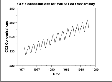
The initial run sequence plot of the data indicates a rising trend. A visual inspection of this plot indicates that a simple linear fit should be sufficient to remove this upward trend.

This plot also shows periodical behavior. This is discussed in the next section.

Linear Trend Removed

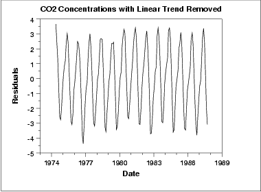
This plot contains the residuals from a linear fit to the original data. After removing the linear trend, the run sequence plot indicates that the data have a constant location and variance, although the pattern of the residuals shows that the data depart from the model in a systematic way.