2. Measurement Process Characterization
2.3. Calibration
2.3.6. Instrument calibration over a regime
2.3.6.7. Uncertainties of calibrated values

2.3.6.7.3.

Comparison of check standard analysis and propagation of error

Propagation of error for the linear calibration

The analysis of uncertainty for calibrated values from a linear calibration line can be addressed using propagation of error. On the previous page, the uncertainty was estimated from check standard values.

Estimates from calibration data

The calibration data consist of 40 measurements with an optical imaging system on 10 linewidth artifacts. A linear fit to the data gives a calibration curve with the following estimates for the intercept, \(a\), and the slope, \(b\),

Parameter  Estimate  Std. Error     t-value      Pr(>|t|)
a         0.2357623  0.02430034    9.702014  7.860745e-12
b         0.9870377  0.00344058  286.881171  5.354121e-65

with the following covariance matrix.

         a             b
a   5.905067e-04 -7.649453e-05
b  -7.649453e-05  1.183759e-05

The results shown above can be generated with R code or Dataplot code. The reader can download the data as a text file.

Propagation of error

The propagation of error is performed for the equation $$ X' = \frac{Y'- \hat{a}}{\hat{b}} $$ so that the squared uncertainty of a calibrated value, \(X'\), is $$ \hspace{-.25in}u^2 = \left[ \frac{\partial{X'}}{\partial{Y'}} \right]^2 s_{Y'}^2 \, + \, \left[ \frac{\partial{X'}}{\partial{\hat{a}}} \right]^2 s_{\hat{a}}^2 \, + \, \left[ \frac{\partial{X'}}{\partial{\hat{b}}} \right]^2 s_{\hat{b}}^2 \, + \, 2 \left[ \frac{\partial{X'}}{\partial{\hat{a}}} \right] \left[ \frac{\partial{X'}}{\partial{\hat{b}}} \right] s_{\hat{a}\hat{b}} $$ where $$ \frac{\partial{X'}}{\partial{Y'}} = \frac{1}{\hat{b}} $$ $$ \frac{\partial{X'}}{\partial{\hat{a}}} = \frac{-1}{\hat{b}} $$ $$ \frac{\partial{X'}}{\partial{\hat{b}}} = \frac{-(Y'-\hat{a})}{\hat{b}^{2}} $$ The uncertainty of the calibrated value, \(X'\), $$ \hspace{-.25in}u^2 = \left( \frac{1}{\hat{b}} \right)^2 s_{Y'}^2 \, + \, \left( \frac{-1}{\hat{b}} \right)^2 s_{\hat{a}}^2 \, + \, \left( \frac{-(Y'-\hat{a})}{\hat{b}^{2}} \right)^2 s_{\hat{b}}^2 \, + \, 2 \left( \frac{-1}{\hat{b}} \right) \left( \frac{-(Y'-\hat{a})}{\hat{b}^{2}} \right) s_{\hat{a}\hat{b}} $$ 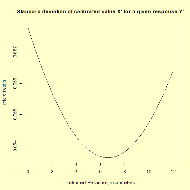is dependent on the value of the instrument reponse \(Y'\).

Graph showing standard deviation of calibrated value X' plotted as a function of instrument response Y' for a linear calibration

Comparison of check standard analysis and propagation of error

Comparison of the analysis of check standard data, which gives a standard deviation of 0.119 μm, and propagation of error, which gives a maximum standard deviation of 0.068 μm, suggests that the propagation of error may underestimate the type A uncertainty. The check standard measurements are undoubtedly sampling some sources of variability that do not appear in the formal propagation of error formula.