1. Exploratory Data Analysis
1.3. EDA Techniques
1.3.6. Probability Distributions
1.3.6.6. Gallery of Distributions

1.3.6.6.19.

Poisson Distribution

Probability Mass Function

The Poisson distribution is used to model the number of events occurring within a given time interval.

The formula for the Poisson probability mass function is

\( p(x;\lambda) = \frac{e^{-\lambda}\lambda^{x}} {x!} \mbox{ for } x = 0, 1, 2, \cdots \)

λ is the shape parameter which indicates the average number of events in the given time interval.

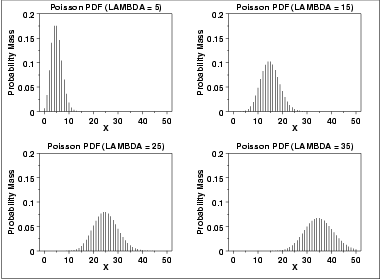
The following is the plot of the Poisson probability density function for four values of λ.

Cumulative Distribution Function

The formula for the Poisson cumulative probability function is

\( F(x;\lambda) = \sum_{i=0}^{x}{\frac{e^{-\lambda}\lambda^{i}} {i!}} \)

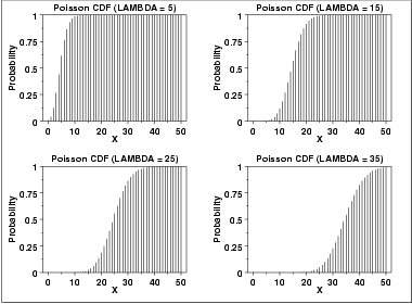
The following is the plot of the Poisson cumulative distribution function with the same values of λ as the pdf plots above.

Percent Point Function

The Poisson percent point function does not exist in simple closed form. It is computed numerically. Note that because this is a discrete distribution that is only defined for integer values of x, the percent point function is not smooth in the way the percent point function typically is for a continuous distribution.

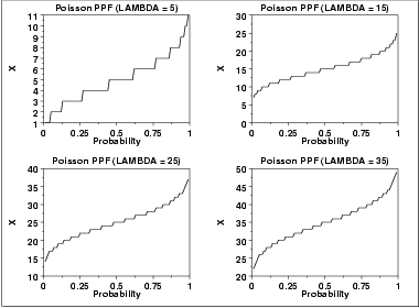
The following is the plot of the Poisson percent point function with the same values of λ as the pdf plots above.

Common Statistics

Mean	λ
Mode	For non-integer λ, it is the largest integer less than λ. For integer λ, x = λ and x = λ - 1 are both the mode.
Range	0 to \(\infty\)
Standard Deviation	\( \sqrt{\lambda} \)
Coefficient of Variation	\( \frac{1} {\sqrt{\lambda}} \)
Skewness	\( \frac{1} {\sqrt{\lambda}} \)
Kurtosis	\( 3 + \frac{1} {\lambda} \)

Parameter Estimation

The maximum likelihood estimator of λ is

\(\tilde{\lambda} = \bar{X}\)

where \(\bar{X}\) is the sample mean.

Software

Most general purpose statistical software programs support at least some of the probability functions for the Poisson distribution.