1.3. EDA Techniques
1.3.5. Quantitative Techniques
1.3.5.18. Yates Algorithm
1.3.5.18.2. |
Important Factors |
- We want the model to include all important factors.
- We want the model to be parsimonious. That is, the model should be as simple as possible.
Seven criteria are utilized to define important factors. These seven criteria are not all equally important, nor will they yield identical subsets, in which case a consensus subset or a weighted consensus subset must be extracted. In practice, some of these criteria may not apply in all situations.
These criteria will be examined in the context of the eddy current data set. The parameter estimates computed using least-squares analysis are shown below.
     Parameter    Estimate
     ---------    --------
     Mean          2.65875
     X1            1.55125
     X2           -0.43375
     X1*X2         0.06375
     X3            0.10625
     X1*X3         0.12375
     X2*X3         0.14875
     X1*X2*X3      0.07125
In practice, not all of these criteria will be used with every analysis (and some analysts may have additional criteria). These critierion are given as useful guidelines. Most analysts will focus on those criteria that they find most useful.
-
\( |\hat{\beta_{i}}| > \Delta \)
That is, declare a factor as "important" if the parameter estimate is greater than some a priori declared engineering difference. This implies that the engineering staff have in fact stated what a minimum difference will be. Oftentimes this is not the case. In the absence of an a priori difference, a good rough rule for the minimum engineering significant Δ is to keep only those factors whose parameter estimate is greater than, say, 10% of the current production average. In this case, let's say that the average detector has a sensitivity of 2.5 ohms. This would suggest that we would declare all factors whose parameter is greater than 10 % of 2.5 ohms = 0.25 ohm to be significant (from an engineering point of view).
Based on this minimum engineering significant difference criterion, we conclude that we should keep two terms: X1 and X2.
-
\( |\hat{\beta_{i}}| < 0.10 \cdot \max |\hat{\beta_{i}}| \)
Based on the order-of-magnitude criterion, we thus conclude that we should keep two terms: X1 and X2. A third term, X2*X3 (0.14875), is just slightly under the cutoff level, so we may consider keeping it based on the other criterion.
-
\( |\hat{\beta_i}| > 2 \cdot \mbox{s.e.}(\hat{\beta_i}) \)
The "2" comes from normal theory (more specifically, a value of 1.96 yields a 95 % confidence interval). More precise values would come from t-distribution theory.
The difficulty with this is that in order to invoke this criterion we need the standard deviation, σ of an observation. This is problematic because
- the engineer may not know σ;
- the experiment might not have replication, and so a model-free estimate of σ is not obtainable;
- obtaining an estimate of σ by assuming the sometimes employed assumption of ignoring 3-term interactions and higher may be incorrect from an engineering point of view.
- the engineer did not know σ;
- the design (a 23 full factorial) did not have replication;
- ignoring 3-term interactions and higher interactions leads to an estimate of σ based on omitting only a single term: the X1*X2*X3 interaction.
This results in keeping three terms: X1 (1.55125), X2 (-0.43375), and X1*X2 (0.14875).
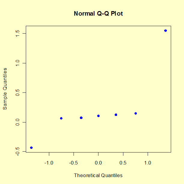
- Normal Probability Plot: Keep a factor as "important" if it
is well off the line through zero on a normal probability
plot of the parameter estimates.
- Half-Normal Probability Plot: Keep a factor as "important" if it is well off the line near zero on a half-normal probability plot of the absolute value of parameter estimates.
Since the half-normal probability plot is only concerned with parmeter magnitudes as opposed to signed parameters (which are subject to the vagaries of how the initial factor codings +1 and -1 were assigned), the half-normal probability plot is preferred by some over the normal probability plot.

For the example at hand, the probability plot clearly shows two factors (X1 and X2) displaced off the line. All of the remaining five parameters are behaving like random drawings from a normal distribution centered at zero, and so are deemed to be statistically non-significant. In conclusion, this rule keeps two factors: X1 (1.55125) and X2 (-0.43375).

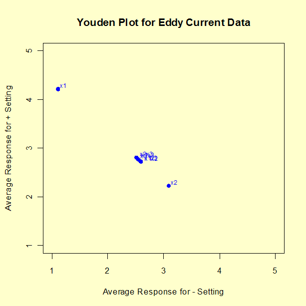
For the example at hand, the Youden plot clearly shows a cluster of points near the grand average (2.65875) with two displaced points above (factor 1) and below (factor 2). Based on the Youden plot, we conclude to keep two factors: X1 (1.55125) and X2 (-0.43375).
-
Residual Standard Deviation > Cutoff
This criterion is different from the others in that it is model focused. In practice, this criterion states that starting with the largest parameter, we cumulatively keep adding terms to the model and monitor how the residual standard deviation for each progressively more complicated model becomes smaller. At some point, the cumulative model will become complicated enough and comprehensive enough that the resulting residual standard deviation will drop below the pre-specified engineering cutoff for the residual standard deviation. At that point, we stop adding terms and declare all of the model-included terms to be "important" and everything not in the model to be "unimportant".
This approach implies that the engineer has considered what a minimum residual standard deviation should be. In effect, this relates to what the engineer can tolerate for the magnitude of the typical residual (the difference between the raw data and the predicted value from the model). In other words, how good does the engineer want the prediction equation to be. Unfortunately, this engineering specification has not always been formulated and so this criterion can become moot.
In the absence of a prior specified cutoff, a good rough rule for the minimum engineering residual standard deviation is to keep adding terms until the residual standard deviation just dips below, say, 5 % of the current production average. For the eddy current data, let's say that the average detector has a sensitivity of 2.5 ohms. Then this would suggest that we would keep adding terms to the model until the residual standard deviation falls below 5 % of 2.5 ohms = 0.125 ohms.
                                                            Residual
Model                                                      Std. Dev.
-----------------------------------------------------      ---------
Mean + X1                                                    0.57272
Mean + X1 + X2                                               0.30429
Mean + X1 + X2 + X2*X3                                       0.26737
Mean + X1 + X2 + X2*X3 + X1*X3                               0.23341
Mean + X1 + X2 + X2*X3 + X1*X3 + X3                          0.19121
Mean + X1 + X2 + X2*X3 + X1*X3 + X3 + X1*X2*X3               0.18031
Mean + X1 + X2 + X2*X3 + X1*X3 + X3 + X1*X2*X3 + X1*X2            NA
Based on the minimum residual standard deviation criteria, and
we would include all terms in order to drive the
residual standard deviation below 0.125. Again, the 5 % rule is a
rough-and-ready rule that has no basis in engineering or
statistics, but is simply a "numerics". Ideally, the engineer has
a better cutoff for the residual standard deviation that is based
on how well he/she wants the equation to peform in practice. If
such a number were available, then for this criterion and data set
we would select something less than the entire collection of terms.
-
Residual Standard Deviation >
σ
That is, declare a term as "important" until the cumulative model that includes the term has a residual standard deviation smaller than σ. In essence, we are allowing that we cannot demand a model fit any better than what we would obtain if we had replicated data; that is, we cannot demand that the residual standard deviation from any fitted model be any smaller than the (theoretical or actual) replication standard deviation. We can drive the fitted standard deviation down (by adding terms) until it achieves a value close to σ, but to attempt to drive it down further means that we are, in effect, trying to fit noise.
In practice, this criterion may be difficult to apply because
- the engineer may not know σ;
- the experiment might not have replication, and so a model-free estimate of σ is not obtainable.
For the current case study:
- the engineer did not know σ;
- the design (a 23 full factorial) did not have replication. The most common way of having replication in such designs is to have replicated center points at the center of the cube ((X1,X2,X3) = (0,0,0)).
Thus for this current case, this criteria could not be used to yield a subset of "important" factors.
|
X1, X2 |
|
X1, X2 |
|
X1, X2, X2*X3 |
|
X1, X2 |
|
X1, X2 |
|
all 7 terms |
|
not applicable |
Such conflicting results are common. Arguably, the three most important criteria (listed in order of most important) are:
|
X1, X2 |
|
X1, X2 |
|
all 7 terms |
Scanning all of the above, we thus declare the following consensus for the eddy current data:
- Important Factors: X1 and X2
- Parsimonious Prediction Equation:
-
\( \hat{Y} = 2.65875 + 1.55125 \cdot X_1 - 0.43375 \cdot X_2 \)
(with a residual standard deviation of 0.30429 ohms)

