1.3. EDA Techniques
1.3.3. Graphical Techniques: Alphabetic
1.3.3.8. |
Complex Demodulation Amplitude Plot |
Detect Changing Amplitude in Sinusoidal Models
-
\[ Y_{i} = C + \alpha\sin{(2\pi\omega t_{i} + \phi)} + E_{i} \]
The complex demodulation amplitude plot (Granger, 1964) is used to determine if the assumption of constant amplitude is justifiable. If the slope of the complex demodulation amplitude plot is not zero, then the above model is typically replaced with the model:
-
\[ Y_{i} = C + \alpha_{i}\sin{(2\pi\omega t_{i} + \phi)} + E_{i} \]
-
\[ Y_{i} = C + (B_0 + B_1*t_{i})
\sin{(2\pi\omega t_{i} + \phi)} + E_{i} \]

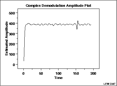
This complex demodulation amplitude plot of the LEW.DAT data set shows that:
- the amplitude is fixed at approximately 390;
- there is a start-up effect; and
- there is a change in amplitude at around x = 160 that should be investigated for an outlier.
- Vertical axis: Amplitude
- Horizontal axis: Time
- Does the amplitude change over time?
- Are there any outliers that need to be investigated?
- Is the amplitude different at the beginning of the series (i.e., is there a start-up effect)?
Assumption Checking
-
\[ Y_{i} = C + \alpha\sin{(2\pi\omega t_{i} + \phi)} + E_{i} \]
The complex demodulation amplitude plot can be used to verify this assumption. If the slope of this plot is essentially zero, then the assumption of constant amplitude is justified. If it is not, α should be replaced with some type of time-varying model. The most common cases are linear (B0 + B1*t) and quadratic (B0 + B1*t + B2*t2).
Complex Demodulation Phase Plot
Non-Linear Fitting

