1.3. EDA Techniques
1.3.3. Graphical Techniques: Alphabetic
1.3.3.10. Contour Plot
1.3.3.10.1. |
DOE Contour Plot |
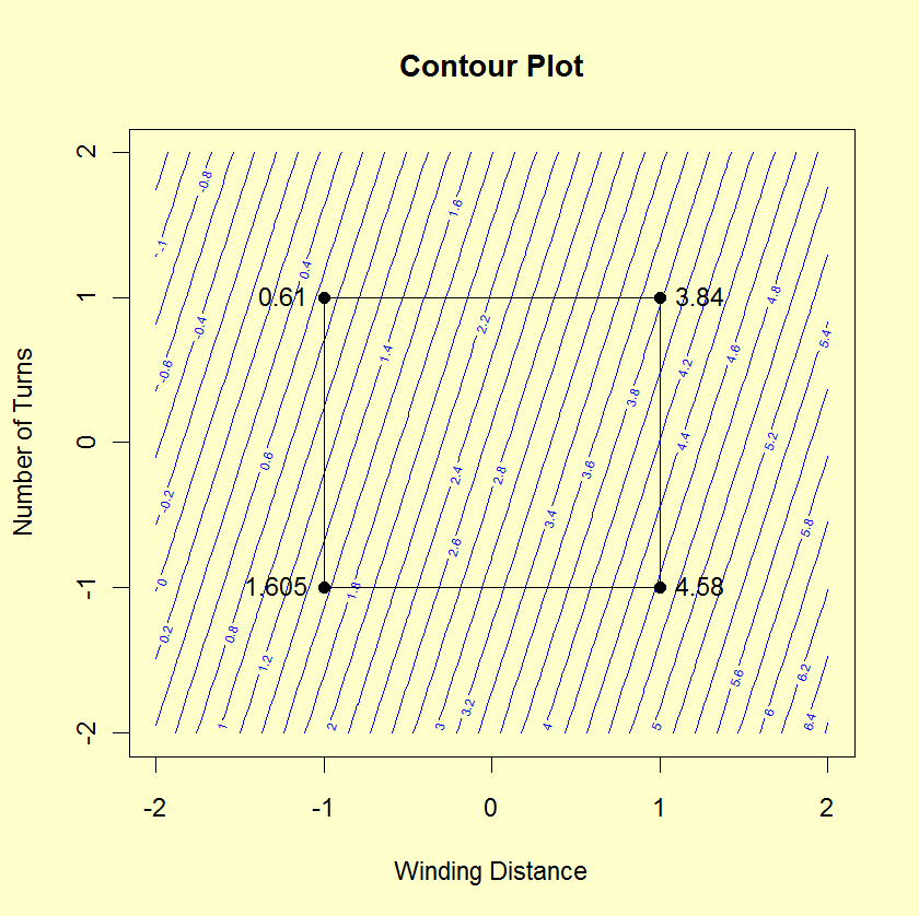
The DOE contour plot is generated for two factors. Typically, this would be the two most important factors as determined by previous analyses (e.g., through the use of the DOE mean plots and an analysis of variance). If more than two factors are important, you may want to generate a series of DOE contour plots, each of which is drawn for two of these factors. You can also generate a matrix of all pairwise DOE contour plots for a number of important factors (similar to the scatter plot matrix for scatter plots).
The typical application of the DOE contour plot is in determining settings that will maximize (or minimize) the response variable. It can also be helpful in determining settings that result in the response variable hitting a pre-determined target value. The DOE contour plot plays a useful role in determining the settings for the next iteration of the experiment. That is, the initial experiment is typically a fractional factorial design with a fairly large number of factors. After the most important factors are determined, the DOE contour plot can be used to help define settings for a full factorial or response surface design based on a smaller number of factors.
- The x and y axes of the plot represent the
values of the first and second factor (independent)
variables.
- The four vertex points are drawn. The vertex points are
(-1,-1), (-1,1), (1,1), (1,-1). At each vertex point,
the average of all the response values at that vertex
point is printed.
- Similarly, if there are center points, a point is drawn
at (0,0) and the average of the response values at the
center points is printed.
- The linear DOE contour plot assumes the model:
-
$$Y = \mu + \beta_1 \cdot U_1 + \beta_2 \cdot U_2 +
\beta_{12} \cdot U_1 \cdot U_2 $$
where μ is the overall mean of the response variable. The values of β1, β2, β12, and μ are estimated from the vertex points using least squares estimation.
In order to generate a single contour line, we need a value for Y, say Y0. Next, we solve for U2 in terms of U1 and, after doing the algebra, we have the equation:
-
$$\displaystyle{U_2 = \frac{(Y_0 - \mu) - \beta_1 \cdot U_1}
{\beta_2 + \beta_{12} \cdot U_1}}$$
We generate a sequence of points for U1 in the range -2 to 2 and compute the corresponding values of U2. These points constitute a single contour line corresponding to Y = Y0.
The user specifies the target values for which contour lines will be generated.

- Interaction significance;
- Best (data) setting for these two dominant factors;
As for factor X3, the contour plot provides no best setting information, and so we would resort to other tools: the main effects plot, the interaction effects matrix, or the ordered data to determine optimal X3 settings.

