8. Assessing Product Reliability
8.2. Assumptions/Prerequisites
8.2.2. How do you plot reliability data?

8.2.2.2.

Hazard and cumulative hazard plotting

Cumulative Hazard Plotting has the same purpose as probability plotting

Similar to probability plots, cumulative hazard plots are used for visually examining distributional model assumptions for reliability data and have a similar interpretation as probability plots. The cumulative hazard plot consists of a plot of the cumulative hazard \(H(t_i)\) versus the time \(t_i\) of the \(i\)-th failure. As with probability plots, the plotting positions are calculated independently of the model and a reasonable straight-line fit to the points confirms that the chosen model and the data are consistent. 

Advantages of Cumulative Hazard Plotting

1. It is much easier to calculate plotting positions for multicensored data using cumulative hazard plotting techniques. 
2. The most common reliability distributions, the exponential and the Weibull, are easily plotted. 

Disadvantages of Cumulative Hazard Plotting

1. It is less intuitively clear just what is being plotted. In a probability plot, the cumulative percent failed is meaningful and the resulting straight-line fit can be used to identify times when desired percentages of the population will have failed. The percent cumulative hazard can increase beyond 100 % and is harder to interpret.
2. Normal cumulative hazard plotting techniques require exact times of failure and running times.
3. Since computers are able to calculate K-M estimates for probability plotting, the main advantage of cumulative hazard plotting goes away.

Since probability plots are generally more useful, we will only give a brief description of hazard plotting. 

How to Make Cumulative Hazard Plots

1. Order the failure times and running times for each of the \(n\) units on test in ascending order from 1 to \(n\) The order is called the rank of the unit. Calculate the reverse rank for each unit (reverse rank = \(n - \mbox{rank} + 1\)).
2. Calculate a hazard "value" for every failed unit (do this only for the failed units). The hazard value for the failed unit with reverse rank \(k\) is just \(1/k\).
3. Calculate the cumulative hazard values for each failed unit. The cumulative hazard value corresponding to a particular failed unit is the sum of all the hazard values for failed units with ranks up to and including that failed unit. 
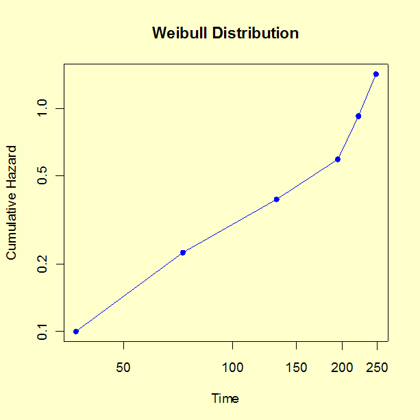
4. Plot the time of failure versus the cumulative hazard value. Linear \(x\) and \(y\) scales are appropriate for an exponential distribution, while a log-log scale is appropriate for a Weibull distribution.

A life test cumulative hazard plotting example

Example: Ten units were tested at high stress test for up to 250 hours. Six failures occurred at 37, 73, 132, 195, 222 and 248 hours. Four units were taken off test without failing at the following run times: 50, 100, 200 and 250 hours. Cumulative hazard values were computed in the following table.

(1) Time of Event	(2) 1= failure 0=runtime	(3) Rank	(4) Reverse Rank	(5) Haz Val (2) x 1/(4)	(6) Cum Hazard Value
37	1	1	10	1/10	.10
50	0	2	9
73	1	3	8	1/8	.225
100	0	4	7
132	1	5	6	1/6	.391
195	1	6	5	1/5	.591
200	0	7	4
222	1	8	3	1/3	.924
248	1	9	2	1/2	1.424
250	0	10	1

Next ignore the rows with no cumulative hazard value and plot column (1) vs column (6).

Plots of example data

Exponential and Weibull Cumulative Hazard Plots

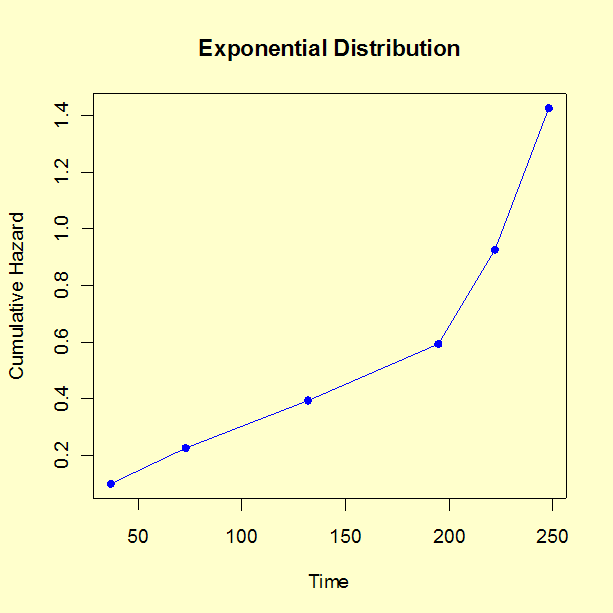
The cumulative hazard for the exponential distribution is just \(H(t) = \alpha t\), which is linear in \(t\) with an intercept of zero. So a simple linear graph of \(y\) = column (6) versus \(x\) = column (1) should line up as approximately a straight line going through the origin with slope \(\lambda\) if the exponential model is appropriate. The cumulative hazard plot for exponential distribution is shown below.

The cumulative hazard for the Weibull distribution is \(H(t) = (t/\alpha)^\gamma\), so a plot of \(y\) versus \(x\) on a log-log scale should resemble a straight line with slope \(\gamma\) if the Weibull model is appropriate. The cumulative hazard plot for the Weibull distribution is shown below. A least-squares regression fit of the data (using base 10 logarithms to transform columns (1) and (6)) indicates that the estimated slope for the Weibull distribution is 1.27, which is fairly similar to the exponential model slope of 1. The Weibull fit looks somewhat better than the exponential fit; however, with a sample of just 10, and only 6 failures, it is difficult to pick a model from the data alone.

Software

The analyses in this section can can be implemented using both Dataplot code and R code.