8. Assessing Product Reliability
8.1. Introduction
8.1.6. What are the basic lifetime distribution models used for non-repairable populations?

8.1.6.1.

Exponential

All the key formulas for using the exponential model

Formulas and Plots

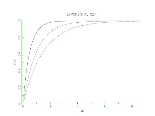
The exponential model, with only one unknown parameter, is the simplest of all life distribution models. The key equations for the exponential are shown below: $$ \begin{array}{ll} \mbox{PDF:} & f(t, \lambda) = \lambda e^{-\lambda t} \\ & \\ \mbox{CDF:} & F(t) = 1-e^{-\lambda t} \\ & \\ \mbox{Reliability:} & R(t) = e^{-\lambda t} \\ & \\ \mbox{Failure Rate:} & h(t) = \lambda \\ & \\ \mbox{Mean:} & \frac{1}{\lambda} \\ & \\ \mbox{Median:} & \frac{\mbox{ln} 2}{\lambda} \cong \frac{0.693}{\lambda} \\ & \\ \mbox{Variance:} & \frac{1}{\lambda^2} \end{array} $$

Note that the failure rate reduces to the constant \(\lambda\) for any time. The exponential distribution is the only distribution to have a constant failure rate. Also, another name for the exponential mean is the Mean Time To Fail or MTTF and we have MTTF = \(1/\lambda\).

The cumulative hazard function for the exponential is just the integral of the failure rate or \(H(t) = \lambda t\).

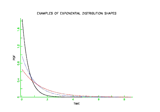
The PDF for the exponential has the familiar shape shown below.

The Exponential distribution "shape"

The Exponential CDF

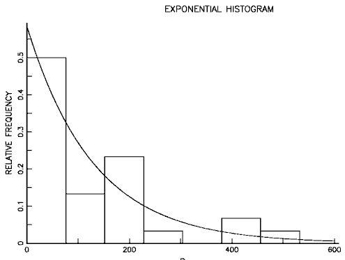
Below is an example of typical exponential lifetime data displayed in Histogram form with corresponding exponential PDF drawn through the histogram.

Histogram of Exponential Data

The Exponential models the flat portion of the "bathtub" curve - where most systems spend most of their "lives"

Uses of the Exponential Distribution Model

1. Because of its constant failure rate property, the exponential distribution is an excellent model for the long flat "intrinsic failure" portion of the Bathtub Curve. Since most components and systems spend most of their lifetimes in this portion of the Bathtub Curve, this justifies frequent use of the exponential distribution (when early failures or wear out is not a concern).
2. Just as it is often useful to approximate a curve by piecewise straight line segments, we can approximate any failure rate curve by week-by-week or month-by-month constant rates that are the average of the actual changing rate during the respective time durations. That way we can approximate any model by piecewise exponential distribution segments patched together.
3. Some natural phenomena have a constant failure rate (or occurrence rate) property; for example, the arrival rate of cosmic ray alpha particles or Geiger counter tics. The exponential model works well for inter arrival times (while the Poisson distribution describes the total number of events in a given period). When these events trigger failures, the exponential life distribution model will naturally apply. 

Exponential probability plot

We can generate a probability plot of normalized exponential data, so that a perfect exponential fit is a diagonal line with slope 1. The probability plot for 100 normalized random exponential observations (\(\lambda\) = 0.01) is shown below.

We can calculate the exponential PDF and CDF at 100 hours for the case where \(\lambda\) = 0.01. The PDF value is 0.0037 and the CDF value is 0.6321.

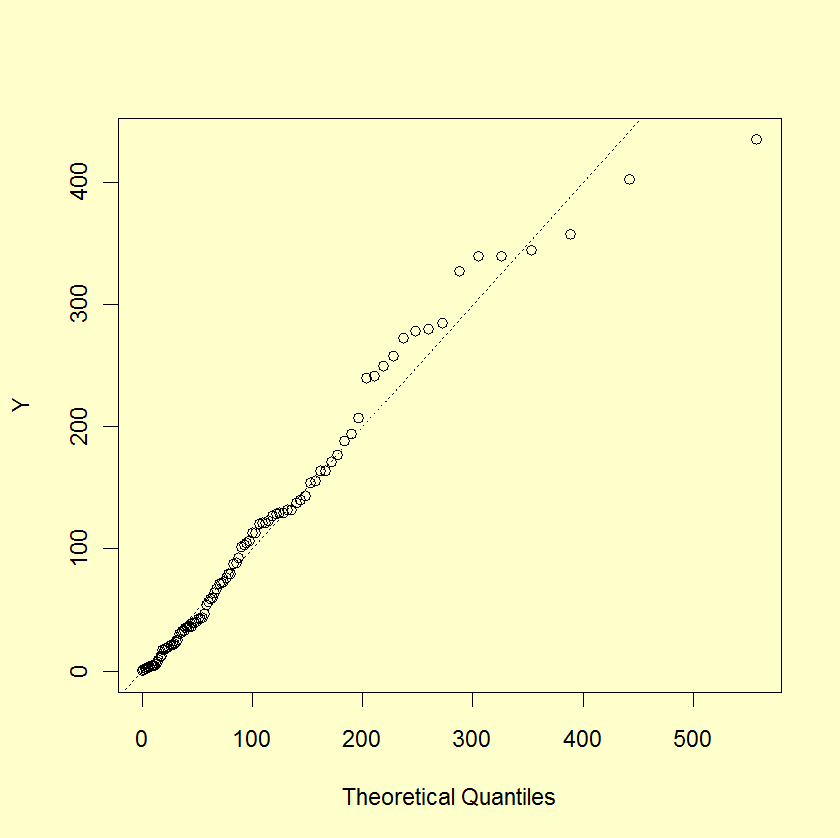
Functions for computing exponential PDF values, CDF values, and for producing probability plots, are found in both Dataplot code and R code.